Tutorial aims:
- What is functional programming
- Building a simple function
- Functions in loops
- Functions with
lapply - Conditional statements
- BONUS: Write a loop to plot multiple graphs
All the resources for this tutorial, including some useful extra reading can be downloaded from this Github repository. Clone and download the repo as a zipfile, then unzip it.
Next, open up a new R Script, preferably in RStudio, where you will write the code for this tutorial. Set the folder you just downloaded as your working directory by running the code below (replacing PATH_TO_FOLDER with the location of the folder on your computer, e.g. ~/Downloads/CC-5-fun-and-loop):
setwd("PATH_TO_FOLDER")
1. Writing functions
We’ve learned how to import data in RStudio, format and manipulate them, write scripts and Markdown reports, how to make beautiful and informative graphs using ggplot2, meaning that you have all the basic tools to perform data simple data analysis using R.
You may find as you work away on your project however, that you want to repeat the same action multiple times. For example, you may want to multiple graphs which differ only in their data input. The temptation is to copy and paste the code multiple times in the script, changing the input dataset each time, but all this copying and pasting increases the chance that you will make a mistake, and it also means that if you want to change some shared element of those copied code chunks, you will have to change each chunk individually.
In this workshop, we introduce the concept of functions and loops in R as a method to minimise the need to copy and paste code chunks, helping to make your code more efficient and readable and minimise the chance of making mistakes by manually retyping code. This tutorial also expands on how to use functions effectively in your code and gives a more formal introduction to functional programming as a coding style.
R is a functional programming language at its heart. When you run a command on some data, e.g. sum(1, 2), sum is a function. Basically everything you do in R involves at least one function. Just as the base R language and other R packages contain functions, you can also write your own functions to perform various tasks using the same tools as package developers, and it’s not as hard as it sounds.
2. Building a simple function
Open a new RStudio session and create a new R script. If you haven’t already done so, download the resources needed for this tutorial from this Github repository. Clone and download the repo as a zipfile, then unzip it. In your R script, set the working directory to the repository you just downloaded by running the code below (replacing PATH_TO_FOLDER with the location of the folder on your computer, e.g. ~/Downloads/CC-5-fun-and-loop):
setwd("PATH_TO_FOLDER")
Let’s import some data from the downloaded repository that we can use to test the function on:
trees_bicuar <- read.csv("trees_bicuar.csv")
trees_mlunguya <- read.csv("trees_mlunguya.csv")
The data contains information on tree stems surveyed in four 1 Ha plots at fieldsites around southern Africa. trees_bicuar contains data for trees in Bicuar National Park in southwest Angola, and trees_mlunguya contains data for trees in southern Mozambique. Each tree stem >5 cm trunk diameter was measured for tree height and trunk diameter, and identified to species.
Have a look at the contents of trees_bicuar before we move on:
head(trees_bicuar)
str(trees_bicuar)
The basic syntax for creating a function looks like this:
example.fn <- function(x, y){
    # Perform an action using x and y
    x + y
}
The function() command is used to tell R that we are creating a function, and we are assigning the function to an object called example.fn. x and y are “arguments” for the function, i.e. things that the user provides when running the function, then in the curly brackets are the actions performed by the function, using the parameters defined by the user earlier in the function call, and any other objects in the working environment in this case adding x and y together.
Run the code above to create the function, then test the function:
example.fn(x = 1, y = 2)
You should get an output of 3, because the function example.fn() was provided with the values of x = 1 and y = 2, which were then passed to the function, which performed the operation x + y. Note that the convention is to name a function using . rather than _ which is normally used to define data objects. This isn’t a rule, but it’s best to stick to the conventions used by other programmers to keep things consistent.
example.fn() is a very simple function, but your functions can be as simple or complex as you need them to be. For example, we can also define a function that calculates the basal area of each stem in m^2 from the diameter, which is in cm. The basal area is the cross-sectional area of the tree trunk if it was cut parallel to the ground.
basal.area <- function(x){
	(pi*(x)^2)/40000
}
This function has one input, x. x can be a numeric vector, or a numeric column in a dataframe, basically anything that doesn’t cause an error in the body of the function. The body of the function multiplies x^2 by pi, then divides by 40,000, giving the basal area as an output.
Test the function by supplying the diameter column from the Bicuar tree stem data (trees_bicuar$diam) to see what the output is:
basal.area(x = trees_bicuar$diam)
Function arguments don’t need to be called x and y, they can be any character string, for example, the function below works identically to the one above, only x is now referred to as dbh:
basal.area <- function(dbh){
	(pi*(dbh)^2)/40000
}
Additionally, you can add a indeterminate number of extra arguments using the ... operator. Imagine that we want to extend our basal.area() function so that it can compute the combined basal area of multiple vectors of diameter measurements, e.g. from multiple sites:
basal.area <- function(...){
    (pi*c(...)^2)/40000
}

basal.area(trees_bicuar$diam, trees_mlunguya$diam)
Just like a normal function, the output of basal.area() can be assigned to a new object, for example, as a new column in trees_bicuar:
trees_bicuar$ba <- basal.area(dbh = trees_bicuar$diam)
Writing functions for simple operations like the example above is useful if you want to perform the same operation multiple times throughout a script and don’t want to copy and paste the same code (e.g. (pi*(dbh)^2)/40000) multiple times, this reduces the chances that you will make a typo when copying and pasting.
3. Functions in loops
We’ve seen how to write a function and how they can be used to create concise re-usable operations that can be applied multiple times in a script without having to copy and paste, but where functions really come into their own is when combined with looping procedures. Loops serve to run the same operation on a group of objects, further minimising the replication of code.
Loops come in two main variants in R, for() loops and while() loops. In this workshop we will focus on for() loops, which are generally easier to read than while() loops, and can be used to perform the same sorts of actions. while() loops are used mainly when the user wants to perform an action a set number of times, whereas a for() loop is generally used when the user wants to perform an action on a named set of objects.
A for() loop iterates through a number of items, most commonly stored as a list, and performs some action equally on each item. It can drastically reduce the amount of copying and pasting.
The basic syntax for creating a for() loop looks like this:
for(i in list){
    # PERFORM SOME ACTION
}
Imagine you have multiple field sites, each with four 1 Ha plots with the tree stem measurements described earlier. The data for each fieldsite is contained in a different dataframe, e.g. trees_bicuar and trees_mlunguya. If we wanted to calculate the basal area for all stems at both sites, we could run:
trees_bicuar$ba <- basal.area(trees_bicuar$diam)
trees_mlunguya$ba <- basal.area(trees_mlunguya$diam)
The above seems fine for now, but what if we had 100 field sites instead of just two? In that case, you can use a for() loop. First, we have to create a list of dataframes to perform the loop on. There are many ways of doing this, but the simplest way is:
trees <- list("trees_bicuar" = trees_bicuar, "trees_mlunguya" = trees_mlunguya)
This makes a list called trees, where each element in the list is a dataframe. List items within a list can be accessed using double square brackets, e.g. trees[[1]] selects the first list item, the dataframe for trees_bicuar. We can take advantage of this method of list indexing using square brackets when we construct our for() loop:
for( i in 1:length(trees) ){
	trees[[i]]$ba <- basal.area(trees[[i]]$diam)
}
The first line sets up the loop, similar to how the function() definition worked earlier. 1:length(trees) creates a sequence of integers from 1 to the length of the list (trees), so in this case the sequence will be 1, 2 as there are two list items. i will take each value of 1:length(trees) in turn, then run the actions in the curly brackets once. For example, the first time the loop runs, i will have a value of 1, and the second time i will have a value of 2. Once the loop has run for the second time, the loop will end, as there are no further values in 1:length(trees).
The body of the loop creates a new column in each dataframe in the list, then runs the function basal.area() using the diam column from the same dataframe as the input. So, the first time the loop runs, it will create a new column called ba in the first list item in trees, trees[[1]].
The above example illustrates how loops work, but often, data are not separated into multiple dataframes from the beginning, instead they are often in a single dataframe with a column to group the different datasets.
Returning to the trees_mlunguya dataset, you can see that there is a column called year, which denotes when each stem measurement was taken. Imagine we want to perform the basal area calculation on each year in the dataset, then find out whether the mean basal area of stems in the plots has changed over the years. We can do this using a for() loop.
First, separate trees_mlunguya into a list of dataframes, each based on the contents of the year column:
trees_mlunguya_list <- split(trees_mlunguya, trees_mlunguya$year)
Then, run a for() loop to fill an empty list with the mean basal area of each year:
# Create an empty list
mean_ba_list <- list()

for( i in 1:length(trees_mlunguya_list) ){
	ba <- basal.area(trees_mlunguya_list[[i]]$diam)
	mean_ba <- mean(ba)
	year <- mean(trees_mlunguya_list[[i]]$year)
	dat <- data.frame(year, mean_ba)
	mean_ba_list[[i]] <- dat
}
During each iteration, this loop creates a number of intermediate data objects (ba, mean_ba, year), and eventually returns a dataframe (dat) with a single row and two columns, one for year and one for mean basal area. Each of these dataframes are then stored as a list item in the new list mean_ba_list.
Of course, this intermediate calculation could be stored in it’s own custom function:
ba.mean.year <- function(dbh, year){
	data.frame(
        mean_ba = mean(basal.area(dbh)),
        year = mean(year)
    )
}

ba.mean.year(trees_mlunguya_list[[1]]$diam, trees_mlunguya_list[[1]]$year)
And this new function can be used in the for loop:
for( i in 1:length(trees_mlunguya_list) ){
	mean_ba_list[[i]] <- ba.mean.year(
		trees_mlunguya_list[[i]]$diam,
		trees_mlunguya_list[[i]]$year)
}
Note that this for() loop now contains a custom function (ba.mean.year()), which itself contains a custom function (basal.area()), demonstrating that there is really no limit to the complexity you can create with functional programming tools like loops and function calls. You can even have loops within loops, and loops in functions!
4. Functions with lapply() family
for() loops are very useful for quickly iterating over a list, but because R prefers to store everything as a new object with each loop iteration, loops can become quite slow if they are complex, or running many processes and many iterations. As an alternative lapply() and the apply family of functions more broadly can be used as an alternative to loops. lapply() runs operations on lists of items, similar to the for() loops above. To replicate the previous for() loop, where we calculated the mean basal area per year in trees_mlunguya, you can run:
lapply(trees_mlunguya_list, function(x){ba.mean.year(dbh = x$diam, year = x$year)})
The first argument of lapply() gives the list object to be iterated over. The second argument defines an unnamed function, where x will be replaced with each list item as lapply() iterates over them. The code inside the curly brackets is the unnamed function, which itself contains our custom function ba.mean.year().
As well as being slightly faster than the for() loop, arguably, lapply is also easier to read than a for() loop.
For another example to illustrate another way lapply() can be used, imagine we wanted to find the mean height of trees in trees_bicuar for each taxonomic family.
First, create a list of vectors of height (rather than dataframes) where each list is a different family of species.
bicuar_height_list <- split(trees_bicuar$height, trees_bicuar$family)
Then run lapply():
lapply(bicuar_height_list, mean, na.rm = TRUE)
Notice how we didn’t have to use curly brackets or an anonymous function, instead, we just passed mean as the second argument of lapply(). I also supplied an argument to mean() simply by specifying it afterwards (na.rm = TRUE).
I could use sapply() to get a more readable output from this loop. sapply() simplifies the output of lapply() to a vector, with elements in the vector named according to the name of the items in the original list:
sapply(bicuar_height_list, mean, na.rm = TRUE)
sapply() won’t be able to simplify the output of every lapply() loop, especially if the output is complex, but for this example, where we only have a single named decimal number, sapply works well.
5. Conditional statements
Another useful functional programming technique is to use conditional statements to change how the code is run depending on whether certain conditions are met. This means that you can create more complex functions that can be applied in a wider range of situations.
For example, in the trees_bicuar data there is a column which refers to the method by which trees_bicuar$height was measured, called trees_bicuar$height_method. One set of field assistants measured tree height with a long stick, while the others had access to a laser range finder, affecting the accuracy with which measurements were taken. Measurements taken with a stick were generally about 1 m short of the actual tree height, while measurements with the laser scanner is only certified accurate to +/- 0.1 m. So a simple correction would be to add 1 m to every measurement done with a stick, and round every measurement done with the laser to the nearest 0.1 m.
A common forestry metric to assess growth of a forest plot over time is “Lorey’s Mean Height”. Lorey’s mean height is calculated by multiplying tree height by the basal area of the tree, then dividing the sum of this calculation by the total plot basal area. We can construct a function which measures Lorey’s mean height for each plot, but we want to adjust the height estimates depending on which method was used. For this, we can use an ifelse() statement.
Basically an ifelse() statement tests for some logical TRUE/FALSE condition in the data, then performs one of two actions depending on the outcome of the test. E.g. “if the value of x is greater than 2, multiply it by 2, else if not, divide by 2”. The code below constructs a function with an ifelse() statement to calculate Lorey’s mean height for the Bicuar plots.
stick.adj.lorey <- function(height, method, ba){
	height_adj <- ifelse(method == "stick", height + 1, round(height, digits = 1))

	lorey_height <- sum(height_adj * ba, na.rm = TRUE) / sum(ba, na.rm = TRUE)

	return(lorey_height)
}
Then we can test the function on each plot using lapply() like we did before:
trees_bicuar_list <- split(trees_bicuar, trees_bicuar$plotcode)

lapply(trees_bicuar_list, function(x){stick.adj.lorey(height = x$height, method = x$height_method, ba = x$ba)})
ifelse() statements can also be used in conjunction with logical TRUE/FALSE function arguments to determine whether certain actions are taken. For example, we can write a function that calculates summary statistics on the trunk diameter measurements for a given fieldsite, and we can use TRUE/FALSE arguments to let the user decide whether certain statistics are calculated:
diam.summ <- function(dbh, mean = TRUE, median = TRUE, ba = TRUE){
		mean_dbh <- ifelse(mean == TRUE,
			mean(dbh),
			NA)
		median_dbh <- ifelse(median == TRUE,
			median(dbh),
			NA)
		mean_ba <- ifelse(ba == TRUE,
			mean(basal.area(dbh)),
			NA)

		return(as.data.frame(na.omit(t(data.frame(mean_dbh, median_dbh, mean_ba)))))
}

diam.summ(dbh = bicuar_trees$diam, mean = TRUE, median = FALSE)
Also note that in this function definition the extra arguments have default values, e.g. mean = TRUE. This means that even if the user doesn’t specify what the value of mean should be, e.g. diam.summ(dbh = trees_bicuar$diam, median = TRUE, mean_ba = FALSE), R will default to the value of mean = TRUE, thus calculating the mean trunk diameter.
6. BONUS: Write a loop to plot multiple graphs
This final section for the workshop provides another real world example using simple for() loops and functions to create multiple graphs of population trends from the Living Planet Index for a number of vertebrate species from 1970 to 2014. Work through the example to make sure that all the code makes sense, remembering the lessons from earlier in the workshop.
First, import the data:
LPI <- read.csv("LPI_data_loops.csv")
You might remember making this scatter plot in the data visualisation tutorial, let’s go through it again for some ggplot2 practice, and to set the scene for our functions later.
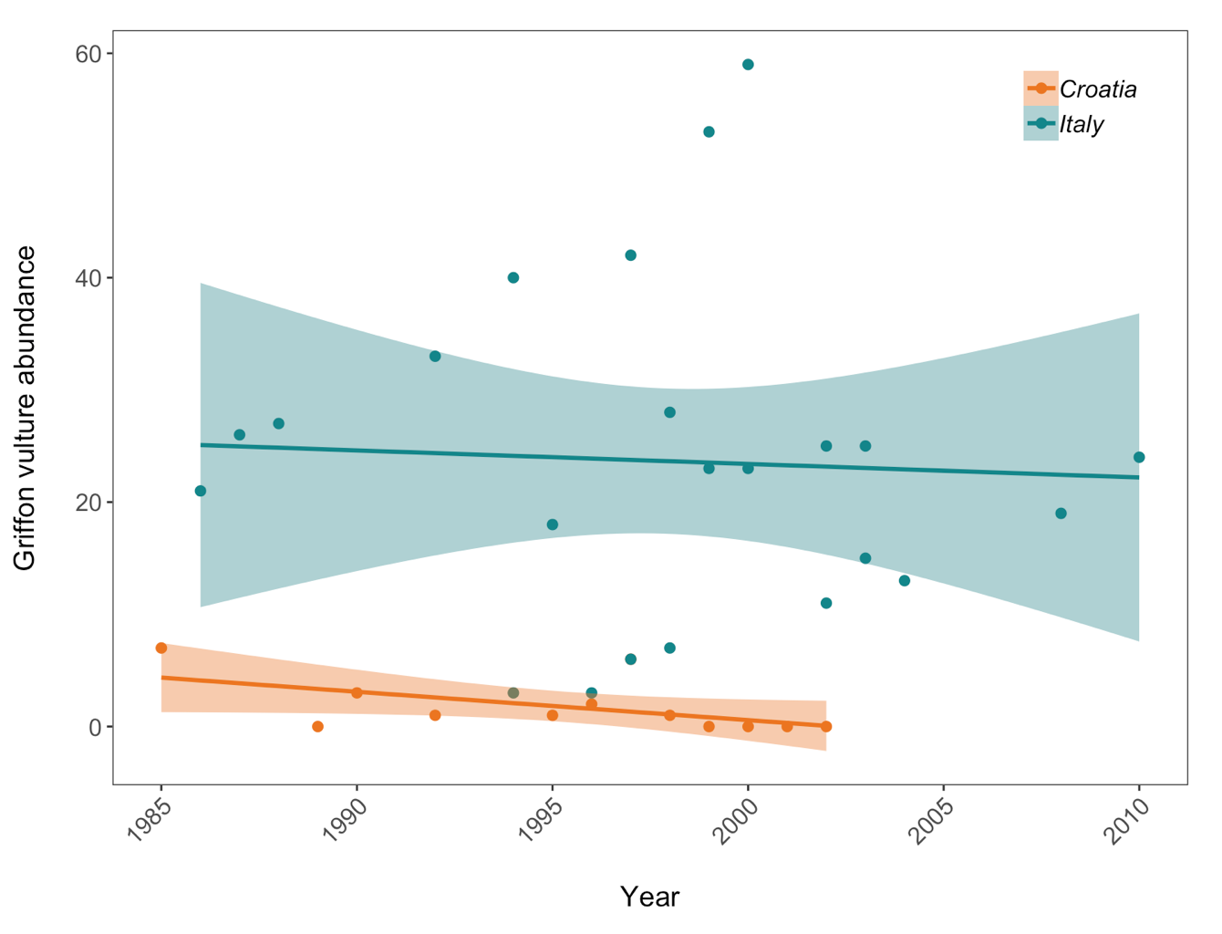
Scatter plot to examine how Griffon vulture populations have changed between 1970 and 2014 in Croatia and Italy:
vulture <- filter(LPI, Common.Name == "Griffon vulture / Eurasian griffon")
vultureITCR <- filter(vulture, Country.list == c("Croatia", "Italy"))

(vulture_scatter <- ggplot(vultureITCR, aes(x = year, y = abundance, colour = Country.list)) +
    geom_point(size = 2) +                                              # Changing point size
    geom_smooth(method = lm, aes(fill = Country.list)) +                # Adding a linear model fit and colour-coding by country
    scale_fill_manual(values = c("#EE7600", "#00868B")) +               # Adding custom colours
    scale_colour_manual(values = c("#EE7600", "#00868B"),               # Adding custom colours
                        labels = c("Croatia", "Italy")) +               # Adding labels for the legend
    ylab("Griffon vulture abundance\n") +
    xlab("\nYear")  +
		theme_bw() +
    theme(axis.text.x = element_text(size = 12, angle = 45, vjust = 1, hjust = 1),       # making the years at a bit of an angle
          axis.text.y = element_text(size = 12),
          axis.title.x = element_text(size = 14, face = "plain"),
          axis.title.y = element_text(size = 14, face = "plain"),
          panel.grid.major.x = element_blank(),                                # Removing the background grid lines
          panel.grid.minor.x = element_blank(),
          panel.grid.minor.y = element_blank(),
          panel.grid.major.y = element_blank(),
          plot.margin = unit(c(0.5, 0.5, 0.5, 0.5), units = , "cm"),           # Adding a 0.5cm margin around the plot
          legend.text = element_text(size = 12, face = "italic"),              # Setting the font for the legend text
          legend.title = element_blank(),                                      # Removing the legend title
          legend.position = c(0.9, 0.9)))               # Setting the position for the legend - 0 is left/bottom, 1 is top/right
Here we are using the theme_bw() theme but we are making lots of modifications to it. When we need to make lots of graphs, e.g. all the graphs for a given research project, we would ideally like to format them in a consistent way - same font size, same layout of the graph panel. That means that we will be repeating many lines of code, but instead of doing that, we can take all the changes we want to make to the ggplot2 theme and combine them into a function of our own! As a reminder, to start writing a function, you first assign it to an object. Since we are making a personalised theme for ggplot2, here I’ve called my function theme.my.own. To tell R that you are writing a function, you use function() and then the commands that you want your function to include go between the {}.
theme.my.own <- function(){
  theme_bw()+
  theme(axis.text.x = element_text(size = 12, angle = 45, vjust = 1, hjust = 1),
        axis.text.y = element_text(size = 12),
        axis.title.x = element_text(size = 14, face = "plain"),
        axis.title.y = element_text(size = 14, face = "plain"),
        panel.grid.major.x = element_blank(),
        panel.grid.minor.x = element_blank(),
        panel.grid.minor.y = element_blank(),
        panel.grid.major.y = element_blank(),
        plot.margin = unit(c(0.5, 0.5, 0.5, 0.5), units = , "cm"),
        plot.title = element_text(size = 20, vjust = 1, hjust = 0.5),
        legend.text = element_text(size = 12, face = "italic"),
        legend.title = element_blank(),
        legend.position = c(0.9, 0.9))
}
Now we can make the same plot, but this time instead of all the code, we can just add + theme.my.own().
(vulture_scatter <- ggplot(vultureITCR, aes (x = year, y = abundance, colour = Country.list)) +
    geom_point(size = 2) +
    geom_smooth(method = lm, aes(fill = Country.list)) +
    theme.my.own() +                                                    # Adding our new theme!
    scale_fill_manual(values = c("#EE7600", "#00868B")) +
    scale_colour_manual(values = c("#EE7600", "#00868B"),
                        labels = c("Croatia", "Italy")) +
    ylab("Griffon vulture abundance\n") +
    xlab("\nYear"))
Remember that putting your entire ggplot code in brackets () creates the graph and then shows it in the plot viewer. If you don’t have the brackets, you’ve only created the object, but haven’t visualized it. You would then have to call the object such that it will be displayed by just typing vulture_scatter after you’ve created the vulture_scatter object.
Let’s make more plots, again using our customised theme.
Filter the data to include only UK populations.
LPI.UK <- filter(LPI, Country.list == "United Kingdom")
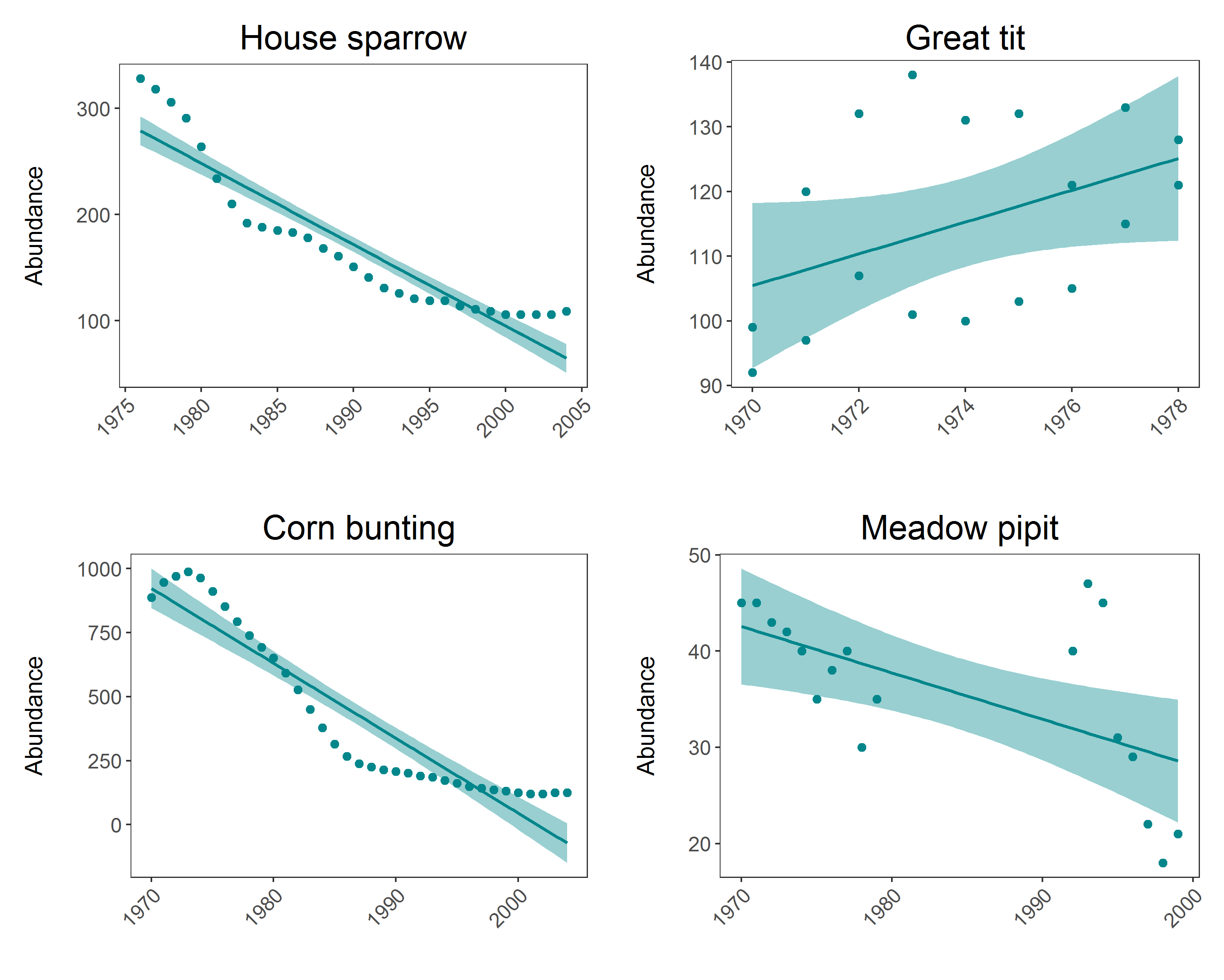
# Pick 4 species and make scatterplots with linear model fits that show how the population has varied through time
# Careful with the spelling of the names, it needs to match the names of the species in the LPI.UK dataframe
house.sparrow <- filter(LPI.UK, Common.Name == "House sparrow")
great.tit <- filter(LPI.UK, Common.Name == "Great tit")
corn.bunting <- filter(LPI.UK, Common.Name == "Corn bunting")
reed.bunting <- filter(LPI.UK, Common.Name == "Reed bunting")
meadow.pipit <- filter(LPI.UK, Common.Name == "Meadow pipit")
Making the plots:
(house.sparrow_scatter <- ggplot(house.sparrow, aes (x = year, y = abundance)) +
    geom_point(size = 2, colour = "#00868B") +
    geom_smooth(method = lm, colour = "#00868B", fill = "#00868B") +
    theme.my.own() +
    labs(y = "Abundance\n", x = "", title = "House sparrow"))

(great.tit_scatter <- ggplot(great.tit, aes (x = year, y = abundance)) +
    geom_point(size = 2, colour = "#00868B") +
    geom_smooth(method = lm, colour = "#00868B", fill = "#00868B") +
    theme.my.own() +
    labs(y = "Abundance\n", x = "", title = "Great tit"))

(corn.bunting_scatter <- ggplot(corn.bunting, aes (x = year, y = abundance)) +
    geom_point(size = 2, colour = "#00868B") +
    geom_smooth(method = lm, colour = "#00868B", fill = "#00868B") +
    theme.my.own() +
    labs(y = "Abundance\n", x = "", title = "Corn bunting"))

(meadow.pipit_scatter <- ggplot(meadow.pipit, aes (x = year, y = abundance)) +
    geom_point(size = 2, colour = "#00868B") +
    geom_smooth(method = lm, colour = "#00868B", fill = "#00868B") +
    theme.my.own() +
    labs(y = "Abundance\n", x = "", title = "Meadow pipit"))
Now arrange all 4 plots in a panel using the gridExtra package and save the file
panel <- grid.arrange(house.sparrow_scatter, great.tit_scatter, corn.bunting_scatter, meadow.pipit_scatter, ncol = 2)
ggsave(panel, file = "Pop_trend_panel.png", width = 10, height = 8)
dev.off() # to close the image
That wasn’t too bad, but you are still repeating lots of code, and here you have only 4 graphs to make - what if you had to make a graph like this for every species in the LPI.UK dataset? That would mean repeating the same code over 200 times. That will be very time consumming, and it’s very easy to make mistakes when you are monotonously copying and pasting for hours.
You might be noticing a pattern in the above ggplot() commands - for every species, we want R to make the same type of graph. We can tell R to do exactly that using a loop!
First we need to make a list of species - we will tell R to make a graph for every item in our list:
Sp_list <- list(house.sparrow, great.tit, corn.bunting, meadow.pipit)
Writing the loop:
for (i in 1:length(Sp_list)) {                                    # For every item along the length of Sp_list we want R to perform the following functions
  data <- as.data.frame(Sp_list[i])                               # Create a dataframe for each species
  sp.name <- unique(data$Common.Name)                             # Create an object that holds the species name, so that we can title each graph
  plot <- ggplot(data, aes (x = year, y = abundance)) +               # Make the plots and add our customised theme
    geom_point(size = 2, colour = "#00868B") +
    geom_smooth(method = lm, colour = "#00868B", fill = "#00868B") +
    theme.my.own() +
    labs(y = "Abundance\n", x = "", title = sp.name)

  ggsave(plot, file = paste(sp.name, ".pdf", sep = ''), scale = 2)       # save plots as .pdf, you can change it to .png if you prefer that

  print(plot)                                                      # print plots to screen
}
The files will be saved in your working directory - to find out where that is, run the code getwd().
Tutorial outcomes:
- You can write a function
- You can write a
for()loop - You understand that loops and functions can be nested to make complex workflows
- You can use
lapply()/sapply()with and without anonymous functions to run loops - You can use conditional
ifelse()statements to make more complex functions
Further reading
Advanced R by Hadley Whickham - Functional Programming