Geospatial vector data in R with sf

Created by Boyan

Content

• Tutorial aims
• 1. Introduction
• 2. OpenStreetMap query
• 3. Coordinate reference systems(CRS)
• 4. Spatial operations
• 5. Draw maps
• 6. Challenge
• Notes
• Further reading
• Bibliography

Tutorial aims

1. Understand the basics of geospatial vector data
2. Learn to obtain geospatial vector data from OpenStreetMap
3. Understand the basics of coordinate reference systems
4. Learn to perform basic spatial operations using the sf library
5. Learn to create simple static (ggplot2) or interactive (tmap).
   

Interactive map produced using tmap. Zoom into Edinburgh to interact with green spaces.

1. Introduction

In this tutorial, you will learn the basics of working with geospatial vector data in R. This tutorial is recommended for learners who have some beginner experience with R and the tidyverse (mainly dplyr, ggplot2 and magrittr pipes (%>%)).

If you are not familiar with some of these, here are some introductory tutorials:

• Intro to R
• Basic data manipulation
• Efficient data manipulation
• Beautiful and informative data visalisation

This tutorial does not require downloading any files. Only an installation of R 4.0+ and the necessary libraries will be needed, as all spatial data we will use will be downloaded directly in the R session.

We highly recommend installing the newest version of R and updating all of the libraries. You check your R version by running the command sessionInfo(). You can easily update all of your libraries from RStudio by going to the “Packages” tab (on the lower-right panel), and clicking on “Update,” then “Select All” and “Install Updates.”

We will use vector data from OpenStreetMap (OSM): a freely accessible, open data online map service. We will use R to obtain certain features we would like to work with: in this tutorial, green spaces in Edinburgh, Scotland. (Data from the query also provided as file in case the query doesn’t work, see the OSM query section.)

We will use the data we get to calculate the area covered by each park and create static and interactive maps, where each type of greenspace is coloured in a different custom colour. We will demonstrate how to transform the data into a different coordinate reference system and how to perform other spatial operations (union and difference between polygons).

The text output of some code chunks is included just under the code chunk, with lines starting with “##”.

What are geospatial vector data?

Geospatial vector data consist of geometries defined based on geographic coordinates. Here are some examples of different geometry types:

• The simplest example is a point geometry, which represents a single point on the Earth’s surface. The locations of different buildings, offices, venues, etc in a city usually take that form.
• A more complex geometry is a linestring, consisting of multiple points connected with each other. Roads, rivers and railways can be represented by linestrings.
• If multiple points are connected to each other to form an enclosed shape, that is a polygon. Any area can be represented by a spatial polygon - a lake, a golf course, or the border of a country.
• There are also multi- geometries for each of the three listed types, consisting of multiple sets of that particular feature. For example, a multipolygon can consist of more than one separate polygon, useful when we want to represent a non-contiguous area.

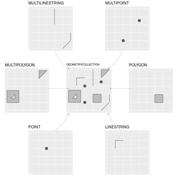
Different classes of simple features geometries. Source: Lovelace et al. (2020) (CC BY-NC-ND 4.0)

This is to be contrasted with raster data, which constist of a matrix of cells (i.e. pixels). An example of raster geographic data is remote sensing imagery. Many maps come in the form of raster images: they do not contain the coordinates of all of the features as they are composed of pixels, and may therefore look pixelated if the resolution is not high enough. However, they usually take less space than vector maps, and can be a faster and more useful map background when the resolution is good. If you are interested rasters, you can read more about the difference between rasters and vectors here, and follow this tutorial to learn how to work with raster data in R.

The sf library

Simple features is a set of standards for geospatial data. The sf library is an implementation of simple features in R.

An sf object in R is based on the dataframe: it has multiple columns with different variables (often called attributes), as well as a geometry column, containing the spatial vector geometry. Each row represents one feature. It also contains information about the coordinate reference system used for the geometries: more on that later.

For a more detailed overview of geographic data in R and the sf library check out Chapter 2 of Geocomputation with R..

Load the R libraries

Let’s load the libraries we need.

# If you don't have any of these, install using:
# install.packages("library_name")

# Load libraries
library(dplyr) # data wrangling
library(tidyr) # data wrangling
library(ggplot2) # data visualisation
library(sf) # simple features - geospatial geometries
library(osmdata) # obtaining OpenStreetMap vector data
library(units) # working with units
library(mapview) # interactive geometry viewing
library(ggmap) # downloading raster maps from a variety of sources
library(ggspatial) # map backgrounds and annotations for ggplot
library(tmap) # static/interactive map library with ggplot-like syntax

Installing the sf library on Windows and Mac OS X should work by running install.packages("sf"). If you use Linux, or have trouble installing it, see this page.

You may get a prompt from R asking whether it should install packages from source. Installing from source rather than binary takes more time, but may give you a slightly newer version. You do not usually need to worry about this and can just respond with “no.”

2. OpenStreetMap query

OpenStreetMap (OSM) provides maps of the world mostly created by volunteers. They are completely free to browse and use, with attribution to © OpenStreetMap contributors and adherence to the ODbL license required, and are used by many public and private organisations. OSM data can be downloaded in vector format and used for our own purposes. In this tutorial, we will obtain data from OSM using a query. A query is a request for data from a database. The Overpass API can be used to perform queries written in the overpass query language, but simple queries can be performed more easily using the osmdata library for R, which automatically constructs the query and imports the data in a convenient format. For this tutorial, we will extract data for the the main types of green spaces in Edinburgh, Scotland: parks, nature reserves, and golf courses.

OSM feature key-value pairs

OpenStreetMap features have attributes in key-value pairs. We can use them to download the specific data we need. These features can easily be explored in the web browser, by using the ‘Query features’ button:

As we can see here, this park has a “name” key with value “The Meadows” and a “leisure” key with the value “park.” If we do further exploration, we see that almost all green spaces in this city have “leisure” equal to either “park,” “nature_reserve,” or “golf_course.” We will request the data for these.

OSM query

First, we start by obtaining the bounding box and polygon for Edinburgh using the getbb() function from the osmdata library.

# Get the polygon for Edinburgh
city_polygon <- getbb("City of Edinburgh",
                      featuretype = "settlement",
                      format_out = "polygon")

# Get the rectangular bounding box
city_rect <- getbb("City of Edinburgh", featuretype = "settlement")

Now, we construct and execute our query:

# Get the data from OSM (might take a few seconds)
greensp_osm <-
  opq(bbox = city_polygon) %>%  # start query, input bounding box
  add_osm_feature(key = "leisure",
                  value = c("park", "nature_reserve", "golf_course")) %>%
  # we want to extract "leisure" features that are park, nature reserve or a golf course
  osmdata_sf() %>%
  # query OSM and return as simple features (sf)
  trim_osmdata(city_polygon)
  # limit data to the Edinburgh polygon instead of the rectangular bounding box

This is a very simple query. We will not go into more details here, but you can read more about osmdata here, and more about more complex overpass queries (that can also easily be executed in R) here.

Let’s have a look at the result of our query.

# Look at query output
greensp_osm

The query returns a list which contains multiple sf object, each for a different geometry type. (We can call individual elements of a list by using list_object$element or list_object[["element"]]). In our results, the polygons and multipolygons are likely of interest. Let’s have a glimpse:

# In our results, polygons and multipolygons are likely of interest. Let's have a look
glimpse(greensp_osm$osm_polygons)
glimpse(greensp_osm$osm_multipolygons)

Here, we see that many columns have been returned, corresponding to all attributes that at least one of the features has. The ‘geometry’ column at the end contains the vector geometries.

Let’s extract them into one sf object. As we have both POLYGON and MULTIPOLYGON features, it would be easiest to convert the POLYGON features to MULTIPOLYGON and then bind the two sf objects. (Polygons can easily be converted to multipolygons without change, while multipolygons may have to be split into multiple features to become polygons.)

We will use the st_cast() to convert the polygon feature to multipolygons, and then bind_rows() to merge them into one sf object. Then, we will use the select() function just like on regular dataframes to keep only columns we need. We will keep the names of the features, their OSM id (in case we would like to refer to them later), and leisure (the type of green space).

# Convert POLYGON to MULTIPOLYGON and bind into one sf object.
greensp_sf <- bind_rows(st_cast(greensp_osm$osm_polygons, "MULTIPOLYGON"),
                                  greensp_osm$osm_multipolygons) %>%
  select(name, osm_id, leisure)

You may notice that we did not put the geometry column into select. That is because in sf features that is not necessary: the select() operation ignores it and so this column is always kept.

Let’s explore the result. First, we can very easily plot the geometries coloured by one of the attributes. In our case, we will use “leisure”.

# Plot coloured by the value of leisure
plot(greensp_sf["leisure"])

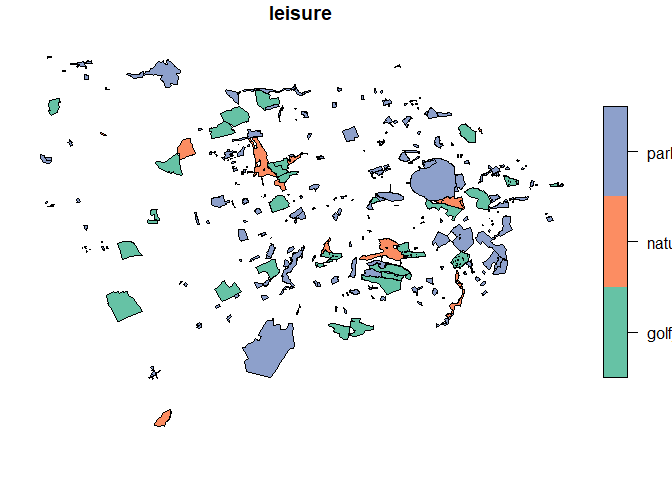
The green spaces in this plot look like the green spaces in Edinburgh on the OSM website, showing us that the query has been successful.

Let’s look at the object.

head(greensp_sf)

    ## Simple feature collection with 6 features and 3 fields
    ## Geometry type: MULTIPOLYGON
    ## Dimension:     XY
    ## Bounding box:  xmin: -3.388398 ymin: 55.90319 xmax: -3.140106 ymax: 55.98513
    ## Geodetic CRS:  WGS 84
    ##                           name  osm_id     leisure                       geometry
    ## 4271400            Dundas Park 4271400        park MULTIPOLYGON (((-3.387083 5...
    ## 4288119     Harrison Park East 4288119        park MULTIPOLYGON (((-3.224193 5...
    ## 4348244      Bruntsfield Links 4348244        park MULTIPOLYGON (((-3.203498 5...
    ## 4891768   Baberton Golf Course 4891768 golf_course MULTIPOLYGON (((-3.28719 55...
    ## 4891786 Kingsknowe Golf Course 4891786 golf_course MULTIPOLYGON (((-3.265052 5...
    ## 4892551                   <NA> 4892551        <NA> MULTIPOLYGON (((-3.146338 5...

Here, we can see the type of geometry of this sf object (MULTIPOLYGON), the coordinate reference system (WGS 84 - more on that in the next section!), and some of the values of each of the columns, including the geometry column. Let’s see the unique values of “leisure”:

unique(greensp_sf$leisure)

## [1] "park"           "golf_course"    NA               "nature_reserve"

The query has returned the three green space types we requested, and for some reason some NA values for “leisure.” Let’s remove these from the object, and rename leisure to greensp_type.

# Filter out unneeded shapes
greensp_sf <-
  greensp_sf %>%
  filter(is.na(leisure) == FALSE) %>%  
  # remove leisure NAs
  rename(greensp_type = leisure) %>%
  # rename leisure to greensp_type
  st_make_valid()
  # a good function to use after importing data to make sure shapes are valid

We have now tidied up our dataset. Here is how we can save it as a file.

Save / load spatial data from file

sf objects can be saved in the form of spatial vector files easily using the st_write() function. It supports multiple geographic data formats. Here’s how it can be saved as a GeoPackage (.gpkg) format, which wraps everything into one file (some formats, such as .shp, create multiple files that need to be kept together). If the file type allows for multiple layers, and we need to specify which layer we want to write our features to.

You can read more about importing/exporting geographic data and different formats in Chapter 7 of Geocomputation with R

st_write(greensp_sf,
         dsn = "greenspaces_Edi_OSM.gpkg", # file path
         layer="greenspaces", # layer name
         layer_options = c(paste0("DESCRIPTION=Contains spatial multipolygons for parks, ",
                                  "nature reserves and golf courses in Edinburgh, Scotland. ",
                                  "Copyright OpenStreetMap constibutors. ODbL ",
                                  "https://www.openstreetmap.org/copyright")),
         # add layer description
         delete_dsn = TRUE
         # to delete the whole file first, because sometimes, we can just
         # overwrite or append one layer to an already existing file.
         # If the file doesn't exist, this will return a friendly warning.
         )

Reading a file is even easier, using st_read():

# If we want to load this dataset:
greensp_sf <- st_read(dsn = "greenspaces_Edi_OSM.gpkg", layer="greenspaces")

3. Coordinate reference systems (CRS)

Coordinate reference systems relate vector geometries to the Earth’s surface, and using the right CRS can be very important to execute our operations successfully. There are two main types of CRS: geographic and projected.

Geographic CRSs identify locations on the Earth using latitude and longitude, in degree units. The surface of the Earth is represented by a sphere or an ellipsoid.

Projected CRSs treat the Earth as a two-dimensional flat surface. All projected CRSs are based on an underlying geographic CRS, as we will see in a bit. The units in a projected CRS are linear, often metres. Projection onto a 2D-surface always introduces some kind of distortion, and the projected CRS we choose can be important depending on our goal.

If you are unfamiliar with projections, this YouTube video illustrates the problem of geographic projection and shows a few commonly used projections.

Let’s have a look at the CRS of our sf object.

st_crs(greensp_sf)

## Coordinate Reference System:
##   User input: EPSG:4326
##   wkt:
## GEOGCRS["WGS 84",
##     DATUM["World Geodetic System 1984",
##         ELLIPSOID["WGS 84",6378137,298.257223563,
##             LENGTHUNIT["metre",1]]],
##     PRIMEM["Greenwich",0,
##         ANGLEUNIT["degree",0.0174532925199433]],
##     CS[ellipsoidal,2],
##         AXIS["geodetic latitude (Lat)",north,
##             ORDER[1],
##             ANGLEUNIT["degree",0.0174532925199433]],
##         AXIS["geodetic longitude (Lon)",east,
##             ORDER[2],
##             ANGLEUNIT["degree",0.0174532925199433]],
##     USAGE[
##         SCOPE["unknown"],
##         AREA["World"],
##         BBOX[-90,-180,90,180]],
##     ID["EPSG",4326]]

Don’t be scared by that output! You don’t need to understand every line to proceed, but some bits are useful. This is called a WKT (well-known text) string, and is one of the methods for describing CRSs. This sf has a geographic CRS - WGS84 (World Geodetic System 84). It is the most commonly used geographic CRS as is used by the Global Positioning System (GPS). Let’s look at some of the elements.

• GEOGCRS["WGS 84" ...] tells us the type of CRS (geographic) and its name.
• DATUM - the underlying model of the Earth’s surface, in this case an ellipsoid.
• CS - coordinate system. It has two axes, geographic latitude and longitude.

The output also gives us the ESPG number of WGS84, which is 4326. The ESPG database contains many CRSs and the ESPG number can be used to refer to a CRS when working with the sf library. Details about different CRSs, including their ESPG number, can be looked up on this website: https://epsg.io/

A lot of spatial operations are done on projected coordinates, and 2D maps of the Earth are by definition projections. For working in a small area of the world, a projected CRS optimised for accuracy for that region would be best. It is also necessary to transform all datasets to the same CRS if they come from different sources.

For example, The British National Grid CRS is very commonly used in Britain. The Ordnance Survey and many other organisations provide geographic data in this format.

Let’s transform our data into the British National Grid CRS, using it’s ESPG number (27700):

greensp_sf <- st_transform(greensp_sf, 27700)

Let’s view the resulting CRS:

# View the CRS
st_crs(greensp_sf)

## Coordinate Reference System:
##   User input: EPSG:27700
##   wkt:
## PROJCRS["OSGB 1936 / British National Grid",
##     BASEGEOGCRS["OSGB 1936",
##         DATUM["OSGB 1936",
##             ELLIPSOID["Airy 1830",6377563.396,299.3249646,
##                 LENGTHUNIT["metre",1]]],
##         PRIMEM["Greenwich",0,
##             ANGLEUNIT["degree",0.0174532925199433]],
##         ID["EPSG",4277]],
##     CONVERSION["British National Grid",
##         METHOD["Transverse Mercator",
##             ID["EPSG",9807]],
##         PARAMETER["Latitude of natural origin",49,
##             ANGLEUNIT["degree",0.0174532925199433],
##             ID["EPSG",8801]],
##         PARAMETER["Longitude of natural origin",-2,
##             ANGLEUNIT["degree",0.0174532925199433],
##             ID["EPSG",8802]],
##         PARAMETER["Scale factor at natural origin",0.9996012717,
##             SCALEUNIT["unity",1],
##             ID["EPSG",8805]],
##         PARAMETER["False easting",400000,
##             LENGTHUNIT["metre",1],
##             ID["EPSG",8806]],
##         PARAMETER["False northing",-100000,
##             LENGTHUNIT["metre",1],
##             ID["EPSG",8807]]],
##     CS[Cartesian,2],
##         AXIS["(E)",east,
##             ORDER[1],
##             LENGTHUNIT["metre",1]],
##         AXIS["(N)",north,
##             ORDER[2],
##             LENGTHUNIT["metre",1]],
##     USAGE[
##         SCOPE["Engineering survey, topographic mapping."],
##         AREA["United Kingdom (UK) - offshore to boundary of UKCS within 49°45'N to 61°N and 9°W to 2°E; onshore Great Britain (England, Wales and Scotland). Isle of Man onshore."],
##         BBOX[49.75,-9,61.01,2.01]],
##     ID["EPSG",27700]]

The description has changed. Some key elements:

• PROJCRS["OSGB 1936 / British National Grid" tells us we now have a Projected CRS, and its name.
• BASEGEOGCRS - as already mentioned, all projected CRSs are based on a geographic CRS. This system is different from WGS84: it has a different ellipsoidal model (DATUM) of the Earth’s surface, which is more accurate for the UK.
• CONVERSION - describes how georgaphic coordinates are converted to projected coordinates. This is a “Transverse Mercator” projection, which is relatively accurate around a central meridian, but gets worse the further east/west you go. Thus, both the datum and the projection are optimised for the UK.
• CS - the axis in this CRS are eastings and northings, and the unit is the metre.

For a more detailed overview of projections and transformations, see Chapter 6 of Geocomputation with R.

4. Spatial operations

Calculate area

Calculating the area of polygon or multipolygon geometries is done using the st_area() function:

# Create and calculate a new column for feature area
greensp_sf <- mutate(greensp_sf, area = st_area(greensp_sf))

Let’s check out the result:

# Look at result
head(greensp_sf$area)

## Units: [m^2]
## [1]  29515.82  29073.37 150754.53 477437.67 398419.52 233094.05

The function has recognised that the coordinate system units in our data are metres, and has returned area as a variable of type units. Using the units library, we can easily convert between measurement units without worrying by how much we need to multiply/divide.

For our purposes, converting to hectares would be more convenient. We can to that using the set_units() function:

# Convert area to to hectares
greensp_sf <- greensp_sf %>%
  mutate(area_ha = set_units(area, "ha")) %>%
  select(-area) # drop area column

Let’s view the resulting sf object interactively. A useful library is mapview, which creates an interactive map with the features, with a popup that shows all of the attributes upon clicking on the feature..

# View interactively
mapview(greensp_sf)

We notice that parks are sometimes overlapped by golf courses or nature reserves. We also notice that some of the green spaces are quite small. Let’s say we want to only keep green spaces that are at least 2 ha.

# Remove green spaces with <2 ha
greensp_sf <- filter(greensp_sf, as.numeric(area_ha) >= 2)

Now, let’s split the sf into multiple sf organised by green space type. This will allows us to easily perform spatial operations between the different types of green space.

# Separate into a list of multiple sf grouped by type
greensp_sf_list <- greensp_sf %>% split(.$greensp_type)

# Each sf object in the list can be accessed using the $ operator.
# E.g. greensp_sf_list$nature_reserve to get the sf object
# containing only nature reserves.

Remove overlap

Let’s say we would like to “cut out” the parts of parks that are covered by golf courses or nature reserves. We need to modify the “park” sf object in our list.

The st_difference(x, y) function will erase the parts of one sf object (x) that are overlapped by another (y). However, to avoid the function comparing each feature in x to each feature in y, we can merge all features in the second sf into one single multipolygon feature using st_union().

# Remove the parts of parks where they are overlapped by nature reserves
greensp_sf_list$park <- st_difference(greensp_sf_list$park,
                                      st_union(greensp_sf_list$nature_reserve))

# Remove the parts of parks where they are overlapped by golf courses
greensp_sf_list$park <- st_difference(greensp_sf_list$park,
                                      st_union(greensp_sf_list$golf_course))

These are only two examples of many possible spatial operations. The sf cheatsheet nicely summarises many of the possible operations.

We can now merge the list back into one sf object. Remember that we changed the features, so we need to calculate area again!

# Let's turn the list back into one sf object. We will also need to re-calculate area!
greensp_sf <- bind_rows(greensp_sf_list) %>%
  # bind the list into one sf object
  mutate(area_ha = set_units(st_area(.), "ha")) %>%
  # calculate area again
  filter(as.numeric(area_ha) >= 2) # remove area < 2 ha again

5. Draw maps

It is now time to draw our maps. First, let’s reorder the types of green spaces in a preferred way, remove underscores and capitalise.

# Reorder greenspace types, capitalise, remove underscores
greensp_sf_forplot <-
  mutate(greensp_sf,
         greensp_type = factor(greensp_type,
                               levels = c("park", "nature_reserve", "golf_course"),
                               labels = c("Park", "Nature reserve", "Golf course")))

Static map with ggplot2 (and ggmap, ggspatial)

We will use the ggmap library to download a raster background for our map. Stamen Maps provide a clean map without too many colours or labels. Always remember to check for license and attribution required! We’ll need to use the rectangular bounding box we obtained at the beginning of the tutorial to download the raster.

# Download Stamen map raster for Edinburgh using ggmap
stamen_raster <- get_stamenmap(city_rect, zoom = 12)

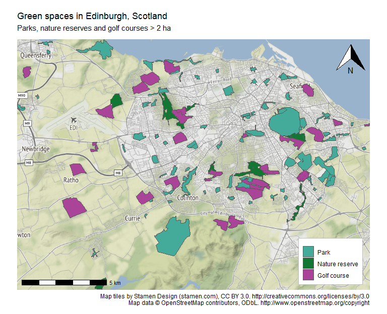
We can now plot using ggplot2:

# Plot map with ggplot
(edi_greenspaces_map <-
  ggplot(data = greensp_sf_forplot) +
    inset_ggmap(stamen_raster) + # add ggmap background
    geom_sf(aes(fill = greensp_type)) + # add sf shapes, coloured by greensp_type
    coord_sf(crs = st_crs(4326), expand = FALSE) +
    # change the CRS of the sf back to WGS84 to match the ggmap raster
    scale_fill_manual(values = c("#44AA99", "#117733", "#AA4499")) +
    # add custom colours from Tol palette (colourblind-friendly)
    labs(title = "Green spaces in Edinburgh, Scotland",
         subtitle = "Parks, nature reserves and golf courses > 2 ha\n",
         caption = paste0("Map tiles by Stamen Design (stamen.com), CC BY 3.0. ",
                         "http://creativecommons.org/licenses/by/3.0\n",
                         "Map data © OpenStreetMap contributors, ODbL. ",
                         "http://www.openstreetmap.org/copyright")) +
    # add various labels
    annotation_scale(location = "bl") + # ggspatial scale on bottom left
    annotation_north_arrow(location = "tr") + # ggspatial arrow on top right
    theme_void() + # get rid of axis ticks, titles
    theme(legend.title = element_blank(),
          legend.position = c(.98, .02),
          legend.justification = c("right", "bottom"),
          legend.box.just = "right",
          legend.box.background = element_rect(fill = "white", colour = "gray"),
          legend.margin = margin(6, 6, 6, 6),
          # move legend to bottom right and customise
          plot.margin = margin(12,12,12,12))
          # add margin around plot
)

This plot can be saved as a file using ggsave():

ggsave("output-maps/edi_greenspaces_map.png", edi_greenspaces_map, width = 8, height = 6.5)

Interactive map with tmap

The tmap library allows us to easily create interactive maps using a ggplot-like syntax.

# Plot interactively with tmap
tmap_mode("view") # interactive mode

(edi_greenspace_tmap <-
  tm_basemap("Stamen.Terrain") + # add Stamen Terrain basemap
  tm_shape(greensp_sf_forplot) + # add the sf
  tm_sf(col = "greensp_type", # colour by green space type
        title = "", # no legend title
        palette = c("#44AA99", "#117733", "#AA4499"), # custom fill colours
        popup.vars = c("Area  " = "area_ha"), # customise popup to show area
        popup.format = list(digits=1)) + # limit area to 1 decimal digit
  tm_scale_bar() # add scale bar
)

This should produce the same interactive map as the one you saw in the beginning of the tutorial (it will appear in the Viewer tab in RStudio). To save the tmap as a .html file:

tmap_save(tm = edi_greenspace_tmap, filename = "output-maps/edi_greenspace_tmap.html")

6. Challenge

Calculate the total area of each type of green space. Please note that we can’t just sum the areas we calculated as there are overlapping polygons within the green space types.

(greensp_type_area <-
  lapply(greensp_sf_list,
      function(x) set_units(st_area(st_union(x)), "ha")) %>% # apply the function to each element of the list using lapply()
  as.data.frame() %>%
  pivot_longer(cols = everything(), names_to = "greensp_type",
               values_to = "area_ha"))

## # A tibble: 3 x 2
##   greensp_type     area_ha
##   <chr>               [ha]
## 1 golf_course     975.6855
## 2 nature_reserve  289.6554
## 3 park           1389.1306

Notes

• Remember that we only extracted three categories of “leisure” form OpenStreetMap for simplicity. There are some other types of green spaces not included in the tutorial. You can practice your skills by expanding the OSM query to include them and then add them to the spatial operations and visualizations.

Further reading

• Geocomputation with R An excellent, free online resource on working with geospatial raster and vector data in R.
• Spatial Data Science (work in progress) Another excellent online book on working with spatial data in R.
• r-spatialecology A collection of R packages for spatial ecology.
• Introduction to Landscape Ecology in R (online slides)

Bibliography

Interesting in learning more about spatial data? Check out our tutorial on raster data and our tutorial on hierarchical modelling of spatial data with R-INLA!