Tutorial aims:
- Introduction and getting started
- Exploring text datasets
- Extracting substrings with regular expressions
- Finding keyword correlations in text data
- Introduction to topic modelling
- Cleaning text data
- Applying topic modelling
- Bonus exercises
1. Introduction
In this tutorial we are going to be performing topic modelling on twitter data to find what people are tweeting about in relation to climate change. From a sample dataset we will clean the text data and explore what popular hashtags are being used, who is being tweeted at and retweeted, and finally we will use two unsupervised machine learning algorithms, specifically latent dirichlet allocation (LDA) and non-negative matrix factorisation (NMF), to explore the topics of the tweets in full.
Prerequisites
- In order to do this tutorial, you should be comfortable with basic Python, the
pandasandnumpypackages and should be comfortable with making and interpreting plots. - You will need to have the following packages installed :
numpy,pandas,seaborn,matplotlib,sklearn,nltk
Getting Started
Twitter is a fantastic source of data for a social scientist, with over 8,000 tweets sent per second. The tweets that millions of users send can be downloaded and analysed to try and investigate mass opinion on particular issues. This can be as basic as looking for keywords and phrases like ‘marmite is bad’ or ‘marmite is good’ or can be more advanced, aiming to discover general topics (not just marmite related ones) contained in a dataset. We are going to do a bit of both.
The first thing we will do is to get you set up with the data.
The data you need to complete this tutorial can be downloaded from this repository. Click on Clone/Download/Download ZIP and unzip the folder, or clone the repository to your own GitHub account.
The original dataset was taken from the data.world website but we have modified it slightly, so for this tutorial you should use the version on our Github.
Import these packages next. You aren’t going to be able to complete this tutorial without them. You are also going to need the nltk package, which we will talk a little more about later in the tutorial.
# packages to store and manipulate data
import pandas as pd
import numpy as np

# plotting packages
import matplotlib.pyplot as plt
import seaborn as sns

# model building package
import sklearn

# package to clean text
import re
Next we will read in this dataset and have a look at it. You should use the read_csv function from pandas to read it in.
df = pd.read_csv('climate_tweets.csv')
Have a quick look at your dataframe, it should look like this:
| tweet | |
|---|---|
| 0 | Global warming report urges governments to act|BRUSSELS, Belgium (AP) - The world faces increased hunger and .. [link] |
| 1 | Fighting poverty and global warming in Africa [link] |
| 2 | Carbon offsets: How a Vatican forest failed to reduce global warming [link] |
| 3 | Carbon offsets: How a Vatican forest failed to reduce global warming [link] |
| 4 | URUGUAY: Tools Needed for Those Most Vulnerable to Climate Change [link] |
Note that some of the web links have been replaced by [link], but some have not. This was in the dataset when we downloaded it initially and it will be in yours. This doesn’t matter for this tutorial, but it always good to question what has been done to your dataset before you start working with it.
2. EDA - Time to start exploring our dataset
Find out the shape of your dataset to find out how many tweets we have. You can use df.shape where df is your dataframe.
One thing we should think about is how many of our tweets are actually unique because people retweet each other and so there could be multiple copies of the same tweet. You can do this using the df.tweet.unique().shape.
You may have seen when looking at the dataframe that there were tweets that started with the letters ‘RT’. Unsurprisingly this is a ReTweet. In the line below we will find how many of the of the tweets start with ‘RT’ and hence how many of them are retweets. We will be doing this with the pandas series .apply method. You can use the .apply method to apply a function to the values in each cell of a column.
We are going to be using lambda functions and string comparisons to find the retweets. If you don’t know what these two methods then read on for the basics.
String Comparisons
String comparisons in Python are pretty simple. Like any comparison we use the == operator in order to see if two strings are the same. For example if
# two string variables for comparison
string1 = 'climate'
string2 = 'climb'
string1 == string2 will evaluate to False.
We can also slice strings to compare their parts, for example string1[:4] == string2[:4] will evaluate to True.
We are going to use this kind of comparison to see if each tweet beings with ‘RT’. If this evaluates to True then we will know it is a retweet.
Lambda Functions
Lambda functions are a quick (and rather dirty) way of writing functions. The format of writing these functions is
my_lambda_function = lambda x: f(x) where we would replace f(x) with any function like x**2 or x[:2] + ' are the first to characters'.
Here is an example of the same function written in the more formal method and with a lambda function
# normal function example
def my_normal_function(x):
    return x**2 + 10
# lambda function example
my_lambda_function = lambda x: x**2 + 10
Try copying the functions above and seeing that they give the same results for the same inputs.
Finding Retweets
Now that we have briefly covered string comparisons and lambda functions we will use these to find the number of retweets. Use the lines below to find out how many retweets there are in the dataset.
# make a new column to highlight retweets
df['is_retweet'] = df['tweet'].apply(lambda x: x[:2]=='RT')
df['is_retweet'].sum()  # number of retweets
You can also use the line below to find out the number of unique retweets
 # number of unique retweets
df.loc[df['is_retweet']].tweet.unique().size
Next we would like to see the popular tweets. We will count the number of times that each tweet is repeated in our dataframe, and sort by the number of times that each tweet appears. Then we will look at the top 10 tweets. You can do this by printing the following manipulation of our dataframe:
# 10 most repeated tweets
df.groupby(['tweet']).size().reset_index(name='counts')\
  .sort_values('counts', ascending=False).head(10)
One of the top tweets will be this one
| tweet | counts | |
|---|---|---|
| 4555 | Take Action @change: Help Protect Wildlife Habitat from Climate Change [link] | 14 |
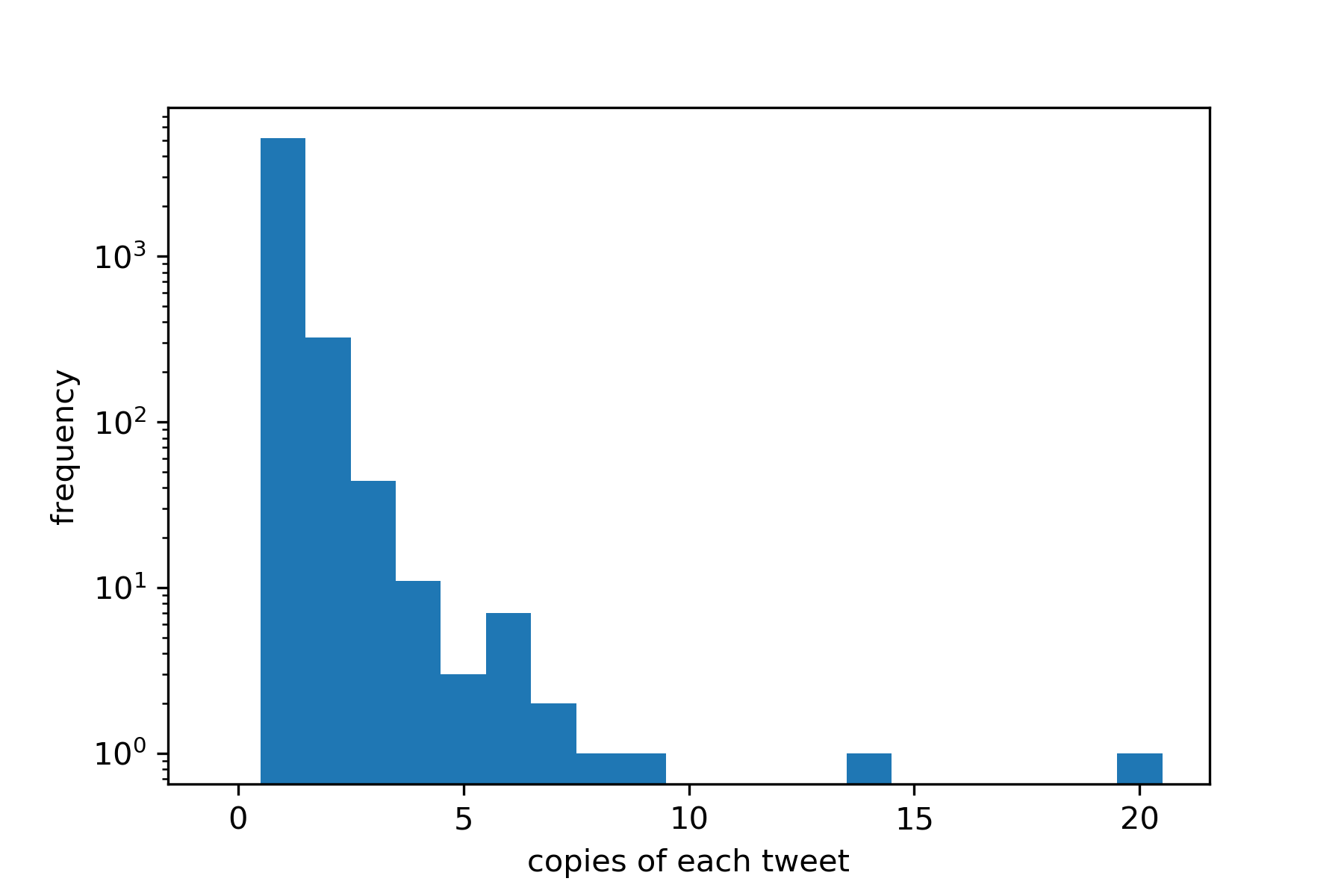
It is informative to see the top 10 tweets, but it may also be informative to see how the number-of-copies of each tweet are distributed. We do that with the following code block.
# number of times each tweet appears
counts = df.groupby(['tweet']).size()\
           .reset_index(name='counts')\
           .counts

# define bins for histogram
my_bins = np.arange(0,counts.max()+2, 1)-0.5

# plot histogram of tweet counts
plt.figure()
plt.hist(counts, bins = my_bins)
plt.xlabels = np.arange(1,counts.max()+1, 1)
plt.xlabel('copies of each tweet')
plt.ylabel('frequency')
plt.yscale('log', nonposy='clip')
plt.show()
3. @who? #what? - Extracting substrings with regular expressions
Next lets find who is being tweeting at the most, retweeted the most, and what are the most common hashtags.
In the following section I am going to be using the python re package (which stands for Regular Expression), which an important package for text manipulation and complex enough to be the subject of its own tutorial. I am therefore going to skim over the details of this package and just leave you with some working code.
If you would like to know more about the re package and regular expressions you can find a good tutorial here on datacamp.
As a quick overview the re package can be used to extract or replace certain patterns in string data in Python. You can use this package for anything from removing sensitive information like dates of birth and account numbers, to extracting all sentences that end in a :), to see what is making people happy.
In this tutorial we are going to be using this package to extract from each tweet:
- who is being retweeted (if any)
- who is being tweeted at/mentioned (if any)
- what hashtags are being used (if any)
Functions to extract each of these three things are below.
def find_retweeted(tweet):
    '''This function will extract the twitter handles of retweed people'''
    return re.findall('(?<=RT\s)(@[A-Za-z]+[A-Za-z0-9-_]+)', tweet)

def find_mentioned(tweet):
    '''This function will extract the twitter handles of people mentioned in the tweet'''
    return re.findall('(?<!RT\s)(@[A-Za-z]+[A-Za-z0-9-_]+)', tweet)

def find_hashtags(tweet):
    '''This function will extract hashtags'''
    return re.findall('(#[A-Za-z]+[A-Za-z0-9-_]+)', tweet)
Try using each of the functions above on the following tweets
# two sample tweets
my_tweet = 'RT @our_codingclub: Can @you find #all the #hashtags?'`
my_other_tweet = 'Not a retweet. All views @my own'
We are now going to make one column in the dataframe which contains the retweet handles, one column for the handles of people mentioned and one columns for the hashtags. We will do this by using the .apply method three times.
Note that each entry in these new columns will contain a list rather than a single value
# make new columns for retweeted usernames, mentioned usernames and hashtags
df['retweeted'] = df.tweet.apply(find_retweeted)
df['mentioned'] = df.tweet.apply(find_mentioned)
df['hashtags'] = df.tweet.apply(find_hashtags)
Print the dataframe again to have a look at the new columns. Your dataframe should now look like this:
| tweet | retweeted | mentioned | hashtags | |
|---|---|---|---|---|
| 36 | RT @virgiltexas: Hey Al Gore: see these tornadoes racing across Mississippi? So much for global "warming" #tornadocot #ocra #sgp #gop #ucot #tlot #p2 #tycot | [@virgiltexas] | [] | [#tornadocot, #ocra, #sgp, #gop, #ucot, #tlot, #p2, #tycot] |
| 37 | #justinbiebersucks and global warming is a farce | [] | [] | [#justinbiebersucks] |
| 297 | Just briefed on global cooling & volcanoes via @abc But I wonder ... if it gets to the stratosphere can it slow/improve global warming?? | [] | [@abc] | [] |
| 298 | Climate Change-ing your Allergies [link] | [] | [] | [] |
4. Keyword Correlations in Text
So far we have extracted who was retweeted, who was mentioned and the hashtags into their own separate columns. Now lets look at these further. We want to know who is highly retweeted, who is highly mentioned and what popular hashtags are going round.
In the following section we will perform an analysis on the hashtags only. We will leave it up to you to come back and repeat a similar analysis on the mentioned and retweeted columns.
First we will select the column of hashtags from the dataframe, and take only the rows where there actually is a hashtag
# take the rows from the hashtag columns where there are actually hashtags
hashtags_list_df = df.loc[
                       df.hashtags.apply(
                           lambda hashtags_list: hashtags_list !=[]
                       ),['hashtags']]
The first few rows of hashtags_list_df should look like this:
| hashtags | |
|---|---|
| 12 | [#Climate, #population] |
| 16 | [#EarthDay] |
| 26 | [#ac] |
| 31 | [#tcot] |
| 36 | [#tornadocot, #ocra, #sgp, #gop, #ucot, #tlot, #p2, #tycot] |
To see which hashtags were popular we will need to flatten out this dataframe. Currently each row contains a list of multiple values. The next block of code will make a new dataframe where we take all the hashtags in hashtags_list_df but give each its own row.
We do this using a list comprehension.
# create dataframe where each use of hashtag gets its own row
flattened_hashtags_df = pd.DataFrame(
    [hashtag for hashtags_list in hashtags_list_df.hashtags
    for hashtag in hashtags_list],
    columns=['hashtag'])
This new dataframe will look like this:
| hashtag | |
|---|---|
| 0 | #Climate |
| 1 | #population |
| 2 | #EarthDay |
Now, as we did with the full tweets before, you should find the number of unique rows in this dataframe. Before this was the unique number of tweets, now the unique number of hashtags.
# number of unique hashtags
flattened_hashtags_df['hashtag'].unique().size
Like before lets look at the top hashtags by their frequency of appearance. You can do this using
# count of appearances of each hashtag
popular_hashtags = flattened_hashtags_df.groupby('hashtag').size()\
                                        .reset_index(name='counts')\
                                        .sort_values('counts', ascending=False)\
                                        .reset_index(drop=True)
A big part of data science is in interpreting our results. Therefore domain knowledge needs to be incorporated to get the best out of the analysis we do. Sometimes this can be as simple as a Google search so lets do that here.
If you do not know what the top hashtag means, try googling it. Does it make sense for this to be the top hashtag in the context of tweets about climate change? Was this top hashtag big at a particular point in time and do you think it would still be the top hashtag today?
Once you have done that, plot the distribution in how often these hashtags appear
# number of times each hashtag appears
counts = flattened_hashtags_df.groupby(['hashtag']).size()\
                              .reset_index(name='counts')\
                              .counts

# define bins for histogram
my_bins = np.arange(0,counts.max()+2, 5)-0.5

# plot histogram of tweet counts
plt.figure()
plt.hist(counts, bins = my_bins)
plt.xlabels = np.arange(1,counts.max()+1, 1)
plt.xlabel('hashtag number of appearances')
plt.ylabel('frequency')
plt.yscale('log', nonposy='clip')
plt.show()
When you finish this section you could repeat a similar process to find who were the top people that were being retweeted and who were the top people being mentioned
From Text to Vector
Now lets say that we want to find which of our hashtags are correlated with each other. To do this we will need to turn the text into numeric form. It is possible to do this by transforming from a list of hashtags to a vector representing which hashtags appeared in which rows. For example if our available hashtags were the set [#photography, #pets, #funny, #day], then the tweet ‘#funny #pets’ would be [0,1,1,0] in vector form.
We will now apply this method to our hashtags column of df. Before we do this we will want to limit to hashtags that appear enough times to be correlated with other hashtags. We can’t correlate hashtags which only appear once, and we don’t want hashtags that appear a low number of times since this could lead to spurious correlations.
In the following code block we are going to find what hashtags meet a minimum appearance threshold. These are going to be the hashtags we will look for correlations between.
# take hashtags which appear at least this amount of times
min_appearance = 10
# find popular hashtags - make into python set for efficiency
popular_hashtags_set = set(popular_hashtags[
                           popular_hashtags.counts>=min_appearance
                           ]['hashtag'])
Next we are going to create a new column in hashtags_df which filters the hashtags to only the popular hashtags. We will also drop the rows where no popular hashtags appear.
# make a new column with only the popular hashtags
hashtags_list_df['popular_hashtags'] = hashtags_list_df.hashtags.apply(
            lambda hashtag_list: [hashtag for hashtag in hashtag_list
                                  if hashtag in popular_hashtags_set])
# drop rows without popular hashtag
popular_hashtags_list_df = hashtags_list_df.loc[
            hashtags_list_df.popular_hashtags.apply(lambda hashtag_list: hashtag_list !=[])]
Next we want to vectorise our the hashtags in each tweet like mentioned above. We do this using the following block of code to create a dataframe where the hashtags contained in each row are in vector form.
# make new dataframe
hashtag_vector_df = popular_hashtags_list_df.loc[:, ['popular_hashtags']]

for hashtag in popular_hashtags_set:
    # make columns to encode presence of hashtags
    hashtag_vector_df['{}'.format(hashtag)] = hashtag_vector_df.popular_hashtags.apply(
        lambda hashtag_list: int(hashtag in hashtag_list))
Print the hashtag_vector_df to see that the vectorisation has gone as expected. For each hashtag in the popular_hashtags column there should be a 1 in the corresponding #hashtag column. It should look something like this:
| popular_hashtags | #environment | #EarthDay | #gop | #snowpocalypse | #Climate | ... | |
|---|---|---|---|---|---|---|---|
| 12 | [#Climate] | 0 | 0 | 0 | 0 | 1 | ... |
| 16 | [#EarthDay] | 0 | 1 | 0 | 0 | 0 | ... |
Now satisfied we will drop the popular_hashtags column from the dataframe. We don’t need it.
hashtag_matrix = hashtag_vector_df.drop('popular_hashtags', axis=1)
In the next code block we will use the pandas.DataFrame inbuilt method to find the correlation between each column of the dataframe and thus the correlation between the different hashtags appearing in the same tweets.
We will use the seaborn package that we imported earlier to plot the correlation matrix as a heatmap
# calculate the correlation matrix
correlations = hashtag_matrix.corr()

# plot the correlation matrix
plt.figure(figsize=(10,10))
sns.heatmap(corrleations,
    cmap='RdBu',
    vmin=-1,
    vmax=1,
    square = True,
    cbar_kws={'label':'correlation'})
plt.show()
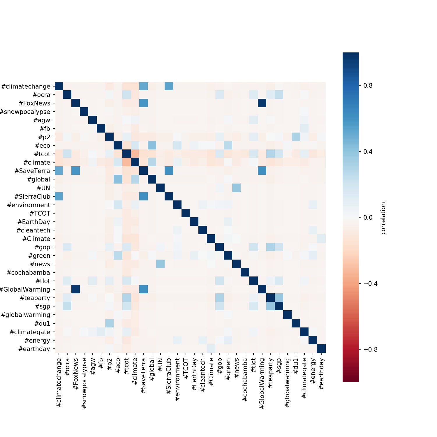
From the plot above we can see that there are fairly strong correlations between:
- #SaveTerra and #SierraClub
- #GloablWarming and #FoxNews
We can also see a fairly strong negative correlation between:
- #tcot and #climate
What these really mean is up for interpretation and it won’t be the focus of this tutorial.
5. Introduction to Topic Modelling
What we have done so far with the hashtags has given us a bit more of an insight into the kind of things that people are tweeting about. We used our correlations to better understand the hashtag topics in the dataset (a kind of dimensionality reduction by looking only at the highly correlated ones). The correlation between #FoxNews and #GlobalWarming gives us more information as a pair than they do separately.
But what about all the other text in the tweet besides the #hashtags and @users? Surely there is lots of useful and meaningful information in there as well? Yes! Absolutely, but we can’t just do correlations like we have done here. There are far too many different words for that! We need a new technique!
…enter topic modelling
Topic modelling is an unsupervised machine learning algorithm for discovering ‘topics’ in a collection of documents. In this case our collection of documents is actually a collection of tweets. We won’t get too much into the details of the algorithms that we are going to look at since they are complex and beyond the scope of this tutorial. We will be using latent dirichlet allocation (LDA) and at the end of this tutorial we will leave you to implement non-negative matric factorisation (NMF) by yourself.
The important information to know is that these techniques each take a matrix which is similar to the hashtag_vector_df dataframe that we created above. Every row represents a tweet and every column represents a word. The entry at each row-column position is the number of times that a given word appears in the tweet for the row, this is called the bag-of-words format. For the word-set [#photography, #pets, #funny, #day], the tweet ‘#funny #funny #photography #pets’ would be [1,1,2,0] in vector form.
Using this matrix the topic modelling algorithms will form topics from the words. Each of the algorithms does this in a different way, but the basics are that the algorithms look at the co-occurrence of words in the tweets and if words often appearing in the same tweets together, then these words are likely to form a topic together. The algorithm will form topics which group commonly co-occurring words. A topic in this sense, is just list of words that often appear together and also scores associated with each of these words in the topic. The higher the score of a word in a topic, the higher that word’s importance in the topic. Each topic will have a score for every word found in tweets, in order to make sense of the topics we usually only look at the top words - the words with low scores are irrelevant.
For example, from a topic model built on a collection on marine research articles might find the topic
- asteroidea, starfish, legs, regenerate, ecological, marine, asexually, …
and the accompanying scores for each word in this topic could be
- 900, 666, 523, 503, 392, 299, 127, …
We can see that this seems to be a general topic about starfish, but the important part is that we have to decide what these topics mean by interpreting the top words. The model will find us as many topics as we tell it to, this is an important choice to make. Too large and we will likely only find very general topics which don’t tell us anything new, too few and the algorithm way pick up on noise in the data and not return meaningful topics. So this is an important parameter to think about.
This has been a rapid introduction to topic modelling, in order to help our topic modelling algorithms along we will first need to clean up our data.
6. Cleaning Unstructured Text Data
The most important thing we need to do to help our topic modelling algorithm is to pre-clean up the tweets. If you look back at the tweets you may notice that they are very untidy, with non-standard English, capitalisation, links, hashtags, @users and punctuation and emoticons everywhere. If we are going to be able to apply topic modelling we need to remove most of this and massage our data into a more standard form before finally turning it into vectors.
In this section I will provide some functions for cleaning the tweets as well as the reasons for each step in cleaning. I won’t cover the specifics of the package we are going to use. The use of the Python nltk package and how to properly and efficiently clean text data could be another full tutorial itself so I hope that this is enough just to get you started.
First we will start with imports for this specific cleaning task.
import nltk
from nltk.tokenize import RegexpTokenizer
from nltk.corpus import stopwords
You will need to use nltk.download('stopwords') command to download the stopwords if you have not used nltk before.
In the cell below I have provided you some functions to remove web-links from the tweets. I don’t think specific web links will be important information, although if you wanted to could replace all web links with a token (a word) like web_link, so you preserve the information that there was a web link there without preserving the link itself. In this case however, we will remove links. We will also remove retweets and mentions. We remove these because it is unlikely that they will help us form meaningful topics.
We would like to know the general things which people are talking about, not who they are talking about or to and not the web links they are sharing.
Extra challenge: modify and use the remove_links function below in order to extract the links from each tweet to a separate column, then repeat the analysis we did on the hashtags. Are there any common links that people are sharing?
def remove_links(tweet):
    '''Takes a string and removes web links from it'''
    tweet = re.sub(r'http\S+', '', tweet) # remove http links
    tweet = re.sub(r'bit.ly/\S+', '', tweet) # rempve bitly links
    tweet = tweet.strip('[link]') # remove [links]
    return tweet

def remove_users(tweet):
    '''Takes a string and removes retweet and @user information'''
    tweet = re.sub('(RT\s@[A-Za-z]+[A-Za-z0-9-_]+)', '', tweet) # remove retweet
    tweet = re.sub('(@[A-Za-z]+[A-Za-z0-9-_]+)', '', tweet) # remove tweeted at
    return tweet
Below we make a master function which uses the two functions we created above as sub functions. This is a common way of working in Python and makes your code tidier and more reusable. The master function will also do some more cleaning of the data.
This following section of bullet points describes what the clean_tweet master function is doing at each step. If you want you can skip reading this section and just use the function for now. You will likely notice some strange words in your topics later, so when you finally generate them you should come back to second last bullet point about stemming.
In the master function we apply these steps in order:
- Strip out the users and links from the tweets but we leave the hashtags as I believe those can still tell us what people are talking about in a more general way.
- After this we make the whole tweet lowercase as otherwise the algorithm would think that the words ‘climate’ and ‘Climate’ were the same. ie it is case sensitive.
- Next we remove punctuation characters, contained in the
my_punctuationstring, to further tidy up the text. We need to do this or we could find tokens* which have punctuation at the end or in the middle. - In the next two steps we remove double spacing that may have been caused by the punctuation removal and remove numbers.
By now the data is a lot tidier and we have only lowercase letters which are space separated. The only punctuation is the ‘#’ in the hashtags.
- Next we change the form of our tweet from a string to a list of words. We also remove stopwords in this step. Stopwords are simple words that don’t tell us very much. Print the
my_stopwordsvariable to see what words we are removing and think whether you can still get the gist of any sentence if you were to take out these words. - In the next step we stem the words in the list. This is essentially where we knock the end off the words. We do this so that similar words will be recognised as the same word by the algorithm. For example in the starfish example we would like it so that the algorithm knows that when it sees ‘regenerate’, ‘regenerated’, ‘regenerates’, ‘regeneration’ or ‘regenerating’ that it will know these are really the same word whilst it is building up topics. It can’t do this itself, so we knock off the word endings so that each of these words will become the same stem - ‘regener’. Once you have copied the
word_rooterfunction, use this line of code to see that these words all become the same thing[word_rooter(w) for w in ['regenerate', 'regenerated', 'regenerates', 'regeneration', 'regenerating', 'regenerative']]. Note that theword_rooterfunction, which is a Porter Stemming function, only uses rules of thumb to know where to cut off words, and so for the word ‘regenerative’ it will actually give it a different root to the other words. - If we decide to use it the next step will construct bigrams from our tweet. This part of the function will group every pair of words and put them at the end. So the sentence
'i scream for ice cream'becomes'i scream for ice cream i_scream scream_for for_ice ice_cream'. A bigram is a word pair like i_scream or ice_cream. The reason for doing this is that when we go from sentence to vector form of the tweets, we will lose the information about word ordering. Therefore we could lose ‘ice cream’ amongst tweets about putting ice and antiseptic cream on a wound (for example). Later we will filter by appearance frequency and so unnatural bigrams like ‘for_ice’ will be thrown out as they won’t appear enough to make it into the most popular tokens*.
* In natural language processing people talk about tokens instead of words but they basically mean the same thing. Here we have 3 kinds of tokens which make it through our cleaning process. We have words, bigrams and #hashtags.
In the next code block we make a function to clean the tweets.
my_stopwords = nltk.corpus.stopwords.words('english')
word_rooter = nltk.stem.snowball.PorterStemmer(ignore_stopwords=False).stem
my_punctuation = '!"$%&\'()*+,-./:;<=>?[\\]^_`{|}~•@'

# cleaning master function
def clean_tweet(tweet, bigrams=False):
    tweet = remove_users(tweet)
    tweet = remove_links(tweet)
    tweet = tweet.lower() # lower case
    tweet = re.sub('['+my_punctuation + ']+', ' ', tweet) # strip punctuation
    tweet = re.sub('\s+', ' ', tweet) #remove double spacing
    tweet = re.sub('([0-9]+)', '', tweet) # remove numbers
    tweet_token_list = [word for word in tweet.split(' ')
                            if word not in my_stopwords] # remove stopwords

    tweet_token_list = [word_rooter(word) if '#' not in word else word
                        for word in tweet_token_list] # apply word rooter
    if bigrams:
        tweet_token_list = tweet_token_list+[tweet_token_list[i]+'_'+tweet_token_list[i+1]
                                            for i in range(len(tweet_token_list)-1)]
    tweet = ' '.join(tweet_token_list)
    return tweet
Use the cleaning function above to make a new column of cleaned tweets. Set bigrams = False for the moment to keep things simple. This is something you could come back to later. Print this new column see if you can understand the gist of what each tweet is about.
df['clean_tweet'] = df.tweet.apply(clean_tweet)
Your new dataframe should look something like this:
| tweet | is_retweet | retweeted | mentioned | hashtags | clean_tweet | |
|---|---|---|---|---|---|---|
| 3 | Carbon offsets: How a Vatican forest failed to reduce global warming [link] | False | [] | [] | [] | carbon offset vatican forest fail reduc global warm |
| 4 | URUGUAY: Tools Needed for Those Most Vulnerable to Climate Change [link] | False | [] | [] | [] | uruguay tool need vulner climat chang |
| 5 | RT @sejorg: RT @JaymiHeimbuch: Ocean Saltiness Shows Global Warming Is Intensifying Our Water Cycle [link] | True | [@sejorg, @JaymiHeimbuch] | [] | [] | ocean salti show global warm intensifi water cycl |
7. Applying Topic Modelling
Good news! We are almost there! Now that we have clean text we can use some standard Python tools to turn the text tweets into vectors and then build a model.
To turn the text into a matrix*, where each row in the matrix encodes which words appeared in each individual tweet. We will also filter the words max_df=0.9 means we discard any words that appear in >90% of tweets. In this dataset I don’t think there are any words that are that common but it is good practice. We will also filter words using min_df=25, so words that appear in less than 25 tweets will be discarded. We discard high appearing words since they are too common to be meaningful in topics. We discard low appearing words because we won’t have a strong enough signal and they will just introduce noise to our model.
* We usually turn text into a sparse matrix, to save on space, but since our tweet database it small we should be able to use a normal matrix.
from sklearn.feature_extraction.text import CountVectorizer

# the vectorizer object will be used to transform text to vector form
vectorizer = CountVectorizer(max_df=0.9, min_df=25, token_pattern='\w+|\$[\d\.]+|\S+')

# apply transformation
tf = vectorizer.fit_transform(df['clean_tweet']).toarray()

# tf_feature_names tells us what word each column in the matric represents
tf_feature_names = vectorizer.get_feature_names()
Check out the shape of tf (we chose tf as a variable name to stand for ‘term frequency’ - the frequency of each word/token in each tweet). The shape of tf tells us how many tweets we have and how many words we have that made it through our filtering process.
Whilst you are here, you should also print tf_feature_names to see what tokens made it through filtering.
Note that the tf matrix is exactly like the hashtag_vector_df dataframe. Each row is a tweet and each column is a word. The numbers in each position tell us how many times this word appears in this tweet.
Next we actually create the model object. Lets start by arbitrarily choosing 10 topics. We also define the random state so that this model is reproducible.
from sklearn.decomposition import LatentDirichletAllocation

number_of_topics = 10

model = LatentDirichletAllocation(n_components=number_of_topics, random_state=0)
model is our LDA algorithm model object. I expect that if you are here then you should be comfortable with Python’s object orientation. If not then all you need to know is that the model object hold everything we need. It holds parameters like the number of topics that we gave it when we created it; it also holds methods like the fitting method; once we fit it, it will hold fitted parameters which tell us how important different words are in different topics. We will apply this next and feed it our tf matrix
model.fit(tf)
Congratulations! You have now fitted a topic model to tweets!
Next we will want to inspect our topics that we generated and try to extract meaningful information from them.
Below I have written a function which takes in our model object model, the order of the words in our matrix tf_feature_names and the number of words we would like to show. Use this function, which returns a dataframe, to show you the topics we created. Remember that each topic is a list of words/tokens and weights
def display_topics(model, feature_names, no_top_words):
    topic_dict = {}
    for topic_idx, topic in enumerate(model.components_):
        topic_dict["Topic %d words" % (topic_idx)]= ['{}'.format(feature_names[i])
                        for i in topic.argsort()[:-no_top_words - 1:-1]]
        topic_dict["Topic %d weights" % (topic_idx)]= ['{:.1f}'.format(topic[i])
                        for i in topic.argsort()[:-no_top_words - 1:-1]]
    return pd.DataFrame(topic_dict)
You can apply this function like so
no_top_words = 10
display_topics(model, tf_feature_names, no_top_words)
Now we have some topics, which are just clusters of words, we can try to figure out what they really mean. Once again, this is a task of interpretation, and so I will leave this task to you.
Here is an example of a few topics I got from my model. Note that your topics will not necessarily include these three.
| Topic 3 words | Topic 3 weights | Topic 4 words | Topic 4 weights | Topic 5 words | Topic 5 weights | |
|---|---|---|---|---|---|---|
| 0 | global | 473.1 | climat | 422.0 | global | 783.0 |
| 1 | warm | 450.7 | chang | 401.8 | warm | 764.7 |
| 2 | believ | 101.3 | legisl | 123.2 | gore | 137.1 |
| 3 | california | 87.1 | us | 105.1 | snow | 123.7 |
| 4 | blame | 82.1 | via | 60.5 | al | 122.1 |
I found that my topics almost all had global warming or climate change at the top of the list. This could indicate that we should add these words to our stopwords like since they don’t tell us anything we didn’t already know. We already knew that the dataset was tweets about climate change.
This result also may have come from the fact that tweets are very short and this particular method, LDA (which works very well for longer text documents), does not work well on shorter text documents like tweets. In the bonus section to follow I suggest replacing the LDA model with an NMF model and try creating a new set of topics. In my own experiments I found that NMF generated better topics from the tweets than LDA did, even without removing ‘climate change’ and ‘global warming’ from the tweets.
8. Bonus
If you want to try out a different model you could use non-negative matrix factorisation (NMF). The work flow for this model will be almost exactly the same as with the LDA model we have just used, and the functions which we developed to plot the results will be the same as well. You can import the NMF model class by using from sklearn.decomposition import NMF.
- Building models on tweets is a particularly hard task for topic models since tweets are very short. Using
len(tweet_string.split(' '))inside a lambda function and feeding this into a.apply, find out the mean value and distribution of how many words there are in each tweet after cleaning? - Try to build an NMF model on the same data and see if the topics are the same? Different models have different strengths and so you may find NMF to be better. You can use
model = NMF(n_components=no_topics, random_state=0, alpha=.1, l1_ratio=.5)and continue from there in your original script.
Further Extension
- If you would like to do more topic modelling on tweets I would recommend the
tweepypackage. This is a Python package that allows you to download tweets from twitter. You have many options of which tweets to download including filtering to a particular area and to a particular time. - Each of the topic models has its own set of parameters that you can change to try and achieve a better set of topics. Go to the sklearn site for the LDA and NMF models to see what these parameters and then try changing them to see how the affects your results.
Summary
Topic modelling is a really useful tool to explore text data and find the latent topics contained within it. We have seen how we can apply topic modelling to untidy tweets by cleaning them first.
Tutorial outcomes:
- You have learned how to explore text datasets by extracting keywords and finding correlations
- You have been introduced to the
repackage and seen how it can be used to manipulate and clean text data - You have been introduced to topic modelling and the LDA algorithm
- You have built you first topic model and visualised the results