Tutorial aims:
Understand why Python is so useful for scientific programming
- Installing Python and running a simple Python program
- Reading data from a file
- Get a feel for how Python looks and feels
- Load data from a text file into memory and basic data structures
- Moving beyond the core Python language with modules
- A brief introduction to data analysis with the pandas package
- Plotting data with Matplotlib
1. Understanding why Python is so useful for scientific programming
You may have heard about the Python programming language before. It is often talked about as the next “up and coming” programming language, or described as being a new, “trendy” programming language that everyone should be learning, particularly scientists. I would argue that Python is no longer merely “up and coming”, or even particularly new, but one of the most popular and useful programming languages you could invest time in learning. In fact, as of 2018, Python is (by certain measures) the most widely used programming language in the world. So if you are a scientist, researcher, or student doing any kind of data analysis, or numeric programming, then I think Python is worth investing some time in learning, even just the basics.
Python is a programming language, a tool used to make computers do useful things for scientific coders much faster than they could do using conventional tools like spreadsheets or plotting software (and certainly much faster than manual calculations!). But programming languages are not really designed for computers at all. In fact, your computer has no idea what all the words and symbols in a piece of code written in Python actually mean. It only understands ones and zeros and electrical currents. Programming languages are actually designed for humans to have a convenient way of programming a computer without getting involved in things like binary and hexadecimal codes, and worrying about electronic circuitry inside the computer.
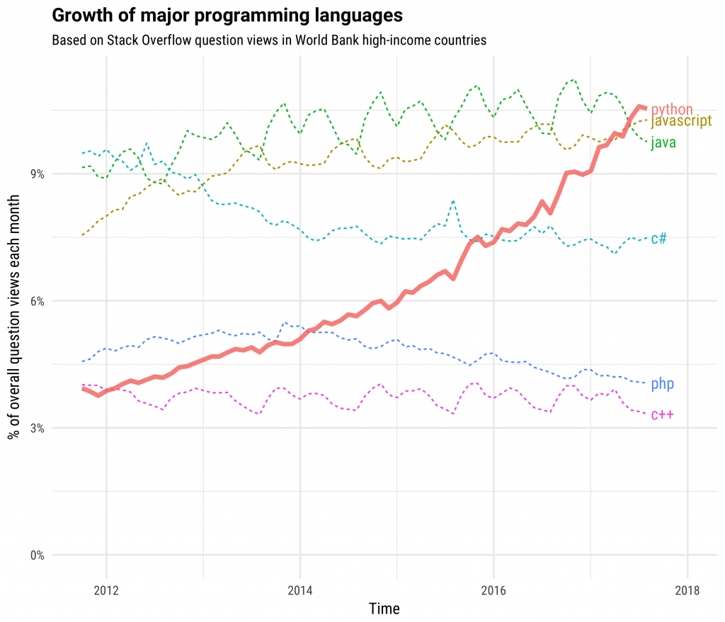
Python has grown hugely in popularity in recent years, by some measures it is the most popular programming language as of 2018. Consider the chart below, which is based on number of question views on StackOverflow:
You may also wish to have a look at this chart showing the growth of Python and other smaller, growing technologies (including R):

If you are interested in reading more about the growth of Python (and the background to the above charts), I highly recommend reading this blog post from StackOverflow.
Python’s strengths as a language
Readability
Python shines because it is designed to be readable by us humans. Python is often described as a language that is intuitive and relatively easy to learn. The syntax (how you arrange the set of words and symbols to make a Python program) is meant to be intuitve to humans by being similar to natural human languages in many ways. For example, look at these little snippets of Python and see if you can guess what they mean and what might happen if we told the computer to run the code:
"Python".startswith("P")
This bit of python code reads like: Python starts with a “P”, and that is exactly what it means in Python!. If we ran this bit of code, the computer would print out True on the screen.
In more technical terms, Python reads the expression (the line of code here) and then evaluates it. It takes the string and checks whether it starts with the letter “P”, by using the function call (or method call) startswith. The expression will either be True or False. This is known as a boolean expression (a true/false expression). The following examples are all examples of boolean expressions.
What about this one?
"thon" in "Python"
If you imagine reading it like a question, if we ask: “thon” in “Python”?, the answer is yes (or True), because the letters “thon” appear in the word “Python”. If we wrote:
"xyz" in "Python"
we would get False, because those letters are not in the word “Python” in that order.
Python syntax has many more similarities with natural languages, and we will discover more throughout this tutorial. Hopefully this will make learning the Python language more intuitive (and fun, as we can compare it to human languages (well, English…)).
Here is one more bonus round. Can you guess what might happen if we ran this Python code? (This will be a bit trickier if you are new to programming, but have a go.)
tastyword = "chocolate"
x = 3

if tastyword.count("o") < x and tastyword.endswith("e"):
  print("You have won some tasty chocolate!")
First we assign the variable tastyword so it refers to the string “chocolate”.
Then we assign the number 3 to the variable x.
Next follows a boolean expression (a true/false question). Actually there are a few boolean expressions here. The first is tastyword.count("o") < x, the second one is tastyword.endswith("e"). This translates to: Count the number of letter o’s in the tastyword variable, and see if it is less than x, and Does the tastyword end with “e”?
Finally there is a logical operator: and. Both boolean expressions in the if statement must be True to allow us to reach the print function. Otherwise nothing will be printed out.
Did you win some chocolate? (I hope so!)
General Purpose
Python has a major advantage when compared to some other commonly used programming languages in the scientific community; it is a general purpose programming language. Compared to other languages such as Matlab, IDL, ncl, and R, which were designed with specific applications in mind, Python was built as a general purpose programming language (like Java, C, Ruby etc.). This means you can use Python to write your data analysis code, plot the results of the analysis, write a numerical model, run a website, do your tax return…the list goes on.
Because of its general-purpose design, Python is used in the real world in a range of industries. Python is used by scientists at universities across the world, developers at big tech companies like Amazon, Facebook, and Google, by financial services companies, and social media apps like Facebook and Instagram, for example. In short, while this tutorial focuses on scientific applications of Python, you are learning a programming language that has a huge variety both within and outwith the scientific community.
Scientific Python Community
The third reason Python is so great is the community behind it. As mentioned before, writing code is as much a way of communicating between humans trying to solve the same scientific problems as it is telling the computer what to do. Python has a very friendly and active community supporting it, many of whom are found on internet resources such as forums and the popular StackOverflow Q&A site.
If you are stuck with a problem in Python, online resources are so plentiful that is often enough to just type “How do I do X in Python”, into a search engine - the first few results often will contain your answer, and often the top link is a StackOverflow question asked by someone with the same or very similar problem to you.
In the domain of science, the Scientific Python community is just as well established. You may have already heard of Python packages like numpy (Numerical Python), scipy (Scientific Python), as well as other tools like pandas, matplotlib, and many more. Many of these tools were developed by scientists to share something back to the Python community, and they have now grown and become almost de facto standard tools within the scientific programming community.
1. Installing Python and running a simple Python program
Installation
The method for installing Python depends on your operating system (Linux/Mac/Windows), but the easiest way I have found, which works across multiple operating systems is to install a distribution of Python called ‘Anaconda’. Anaconda includes a range of useful packages for scientific coding, such as matplotlib, numpy and pandas (We will cover these later on in the tutorial). It all comes with the conda package manager - a tool for easily installing other Python add-on packages that you may want to use. It also comes with a few useful programmes which can be used to write Python code. The download link is here: Downloading Anaconda.
Make sure to install a Python 3 version specific to your operating system
If you are in the ‘live’ workshop, now would be a good point to raise any issues or questions you have about installing Python.
On Windows, you may run into some problems, depending on you version, but help can be found in the official Python documentation pages for using Python on Windows.
The Python workflow
From here you have two main options for how to write your Python code during this workshop:
Option A - Following the tutorial with the command line and any text editor
This method of writing Python code is most applicable to Mac and Linux users, as it requires access to a terminal program like Terminal.app, or the Gnome Terminal.
The way Python programming normally works is that you write a script, save the script, then run the script. Python scripts can be written using any plain text editor, e.g. Atom, PsPad, Vim, or even simple programs like TextEdit.app!
To run the Python script, you then need to navigate to the folder where the Python script is saved, using the command line, and run it by typing this, assuming your Python script is called myscript.py:
python myscript.py
Any output will be printed to the screen in the terminal or console you are running from.
This workshop doesn’t cover the command line/terminal in depth, but handy ‘cheat sheets’ are available here for Linux/Mac terminal users and Windows command line users.
Option B - Following the tutorial with Spyder or another IDE
If you are not comfortable using the command line or terminal, or are on a Windows machine, we recommend using this method.
Instead of using a text editor and the command line, you can write and run your Python scripts using an IDE (Integrated Development Environment) such as Spyder (similar to RStudio). Spyder is bundled with the Anaconda installation, so it should be easily accessible. Ask the workshop helpers for guidance, or consult the Spyder documentation for more info on how to use Spyder.
This diagram shows a basic Spyder session:
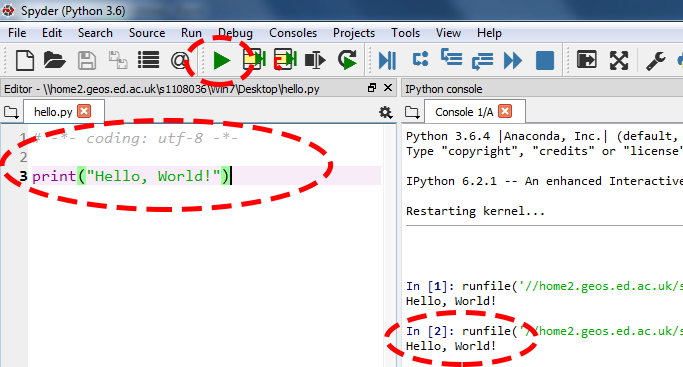
The window on the left is a text editor where you can write your script, the window on the right is the console where the output of the script will be shown. The green play button will run the script through the console, giving you the output.
Although we recommend using Spyder if you are a beginner, there are many other ways to use Python. One notable method is called IPython.
For consistency in this workshop and to maintain transferability between different platforms, the rest of the tutorial assumes that you are using the text editor and command line approach described above, but everything should still work if you want to use an IDE like Spyder.
Hello, World!
Let’s try running the most basic program to test you have a working Python installation:
Open a text file with the editor of your choice or in the Spyder IDE, and type the following lines:
print("Hello, World!")
Then save the file as hello.py.
If you are using the Spyder IDE, you can then press the green play button or select “Run” from the menu to run the script through the console on the right hand side of the screen.
If you are using the command line you can navigate to the folder where hello.py is stored, then run the script by typing:
python hello.py
Hopefully, regardless of what method you use, you should see “Hello, World!” printed to screen.
Files for this tutorial
This short tutorial is based around exploring data from the School of GeoSciences weather station, which is located on top of the James Clark Maxwell Building at the University of Edinburgh.
You can download the data, and some helpful Python cheatsheets from this github repository. Clone and download the repo as a zipfile by pressing the big green button, then unzip it. You should then save any python scripts to that folder, so they can access the data easily.__
Alternatively, you can fork the repository to your own Github account and then clone it using the HTTPS/SSH link. For more details on how to register on Github, download Git and use version control, please check out our previous tutorial.
You can have a look at all the data via the link to the station webpage, but for ease of use, we’ve provided the data file in the repository you just downloaded (StormEleanor_2_3_Jan.csv). Specifically, the data comes from Storm Eleanor, which passed over the UK and Edinburgh on the 2nd-3rd January 2018.
2. Reading data from a file
We are going to start off simple, using the basic ‘core’ Python language features to explore the data, then later in the tutorial we’ll look at some of the ways we can use modules and libraries to make dealing with data easier. Create a new Python script in your editor or IDE, and type in the following lines:
weatherfile = open("StormEleanor_2_3_Jan.csv", "r")

for line in weatherfile:
  print(line)

weatherfile.close()
Save it and run the script. You should see all the lines of the csv file are printed out to screen.
It’s good practice in Python to use a keyword called with when you are reading from (or writing to) data files. The with keyword ensures that files are automatically closed properly at the end of their use, and system resources are correctly freed up. You could think of it intuitively like, “With this file opened as this shorthand name, I am going to do these things in the following block of code…”. The above script can be shortened by replacing the open() and close() statements with a single with and open as below:
with open("StormEleanor_2_3_Jan.csv", "r") as weatherfile:
  for line in weatherfile:
    print(line)
Note how when using with we do not have to worry about closing the file – it is taken care of automatically when we exit the code block. with also makes sure that any exceptions that occur when opening the file are dealt with appropriately.
The second argument we provide to the open() function, "r", tells the Python we want to open the file for reading from it. There are other arguments that we could have given such as "w" for writing to the file. More details can be found in the Python documentation.
3. A note on code blocks in Python
All programming languages need a way of marking small units or subsections of code. For example, in a for loop, there needs to be a way to mark the start and end of the code to be executed within the loop. Some programming languages use terminating keywords to take care of this, Matlab and Fortran for example use the end keyword to signify the end of a particular code block. C-based languages often use the “curly braces” to open and close code blocks. E.g.:
if (some_condition == true):
{
  // do something here inside the braces...
}
Python uses neither braces nor “end” statements to mark the end of code blocks. Instead, the end of code blocks are inferred from the indentation or whitespace. Indenting code in Python implies that you are starting a code block, such as in the for loops or with blocks in the above examples. To end the code block (say at the end of an if statement, you simply un-indent the code to the previous indentation level. This often catches people out when first using Python – Python in this respect is quite a visual language – you need to look at the indentation levels to work out where your code blocks start and finish. There are advantages and disadvantages to this, but one major advantage is that it forces you to write very legible and consistently indented code! Python will complain if your indentation is wrong or inconsistent.
You may use either a tab or spaces (any number of spaces…) to indicate indentation. I prefer personally to use two spaces, as it’s easy to type and keeps the code looking nice and compact, but it’s up to your personal preference. The important thing is to be consistent with your whitespace and indentation!
4. Loading a text file into memory and basic data structures
We can load the data in from the file and print it to screen, but that probably isn’t much practical use. How should we approach reading the data into variables that we can manipulate and perform calculations on? We can do this by assigning the values in the file to a basic Python data structure, the list. (We shall discover later that lists are not necessarily the best data struture for numerical data, but they are a good introduction when learning Python.)
Firstly, our csv file is separated by commas, but we need to get rid of these before we can start doing useful things with the data. In fact, although it is obvious to us that we are dealing with numeric data, Python is just treating the text file as a bunch of lines of text, rather than numbers. In Python (and many other languages), this type of data is refered to as a string. Try changing the print(line) function in the above code snippet to: print(type(line)) and run the program again.
with open("StormEleanor_2_3_Jan.csv", "r") as weatherfile:
  for line in weatherfile:
    print(type(line))
You should get this output printed repeatedly to screen:
<class 'str'>
If you are using the older Python version 2, it will be slightly different:
<type 'str'>
…but it effectively means the same thing.
str is short for string, i.e. text or characters. But wait, this means that the variable line is just one long string of text from our data, including all the commas from the csv file format. This is not ideal if we want to work on individual values from the file. Luckily, Python is very good at manipulating strings. We can break up the data by splitting the string. Change the script so it contains:
with open("StormEleanor_2_3_Jan.csv", "r") as weatherfile:
  for line in weatherfile:
    print(line.split(','))
We should get output that looks something like this:
...
['1239882', '252.5', '3.466666', '4.3', '6.5', '78', '978.0999', '0\n']
...
We also probably want the data separated by the columns, so we can do calculations on each column of data, like wind-speed, rainfall, pressure, and so on.
Let’s suppose we are interested in the air pressure from our data file. Air pressure is stored in the 7th column of the text file. However, Python, like many other programming languages, starts counting from zero, so the columns of each line are numbered 0, 1, 2, 3, 4, 5, 6, 7. So to get the seventh column we actually use the number 6:
with open("StormEleanor_2_3_Jan.csv", "r") as weatherfile:
  for line in weatherfile:
    data_row = line.split(',')
    pressure = data_row[6]
    print(pressure)
We’ve broken this down into stages now. First we create a variable called data_row to store each line of the text file as a list as we read it in. Then we get each value of pressure by indexing the data_row list with the number 6. Finally we print the pressure value to screen. Run the above code and you should get all the pressure values printed out.
This is okay, but we are just printing out values of pressure, not storing them anywhere. In fact we are overwriting the value of pressure every time we go through the for loop. So we are going to create a list of pressure values that we can store and reuse. The script should be changed to look like this:
pressure_data = []

with open("StormEleanor_2_3_Jan.csv", "r") as weatherfile:
  for line in weatherfile:
    data_row = line.split(',')
    pressure = data_row[6]
    pressure_data.append(pressure)
Note that we must first create an empty list to store our pressure data in. We also have to make sure to create it outside of the with block, in case we want to use it later on. In the for loop we do the following for every line:
- Split the line up from one long string into a list of items in the row.
- Extract the item at position 6. (The pressure reading)
- Use the
appendmethod to add the current line’s pressure value to our list of pressure data.
We now have a data structure called pressure_data that contains all the air pressure measurements from the text file. But there are a couple of problems here. (Can you think what they might be?)
Hint - Think about:
- The very first line in the original text file
- The type of the data in the list…
Yes, unfortunately, we have two problems: 1. The first text line in the original file (Pair_avg) has been read into the list, which is not good if we want to try and sum or average the list later, because it will contain a string as well as some numbers. 2. The items in the list are actually all still strings, not numbers! You can test this by adding two print statements to the end of the script:
pressure_data = []

with open("StormEleanor_2_3_Jan.csv", "r") as weatherfile:
  for line in weatherfile:
    data_row = line.split(',')
    pressure = data_row[6]
    pressure_data.append(pressure)

# Oh no! This is the header line!
print(pressure_data[0])   # Prints: 'Pair_avg'

# Argh! This is a string!
print(type(pressure_data[1]))  # Prints: 'str'
Remember that pressure_data[0] refers to the very first line of the csv file we read in, which is a header line containing text. Similarly, pressure_data[1] refers to the second line of the csv file, because Python counts from zero.
No worries, we can fix this. To skip the header line, we can use a handy built-in function in Python called next(). next() can be used on objects or data structures in Python to simply mean “Go to the next item in this object”. By adding next(weatherfile), we are telling Python to take us to the next line before we start to do anything else.
Python is normally quite good at inferring what type of data you are dealing with, but sometimes it needs a hint. We can do this by converting our pressure variable from a string to a floating-point number by doing: float(pressure)
With the above amendments, your script should now look like:
pressure_data = []

with open("StormEleanor_2_3_Jan.csv", "r") as weatherfile:
  next(weatherfile)
  for line in weatherfile:
    data_row = line.split(',')
    pressure = data_row[6]
    pressure_data.append(float(pressure))
If you like you can add print statements to check that the type of data is no longer strings, and that we have skipped over the header line containing the description text.
pressure_data = []

with open("StormEleanor_2_3_Jan.csv", "r") as weatherfile:
  next(weatherfile)
  for line in weatherfile:
    data_row = line.split(',')
    pressure = data_row[6]
    pressure_data.append(float(pressure))

print(pressure_data[0])
print(type(pressure_data[1]))
The output should be:
989.4
<class 'float'>
5. Moving beyond the core Python language with modules
This all seems a bit long-winded, doesn’t it? Isn’t Python meant to be quick and easy, I hear you cry?
Correct. Python’s simple and hopefully intuitive syntax is nice, but the real strength of Python lies in its support for packages and libraries/modules that make your coding life easier.
Python actually has built in support for reading text and csv files, using a module (or library) called…csv! So there is no need to do all of the above every time you want to read in a simple text file. But I hope it was useful introduction to the feel of Python syntax, and some of the basic language features – they will come in handy later!
To use the csv module in Python, we have to import it first, which is just a way of saying we want to bring this module into our Python program and use its features.
import csv

pressure_data = []   # Create an empty list as before to store values

with open('StormEleanor_2_3_Jan.csv', 'r') as csvfile:
  next(csvfile)
  for row in csv.reader(csvfile, quoting=csv.QUOTE_NONNUMERIC):
    pressure_data.append(row[6])

# Check our variables look okay and they are the correct type:
print(pressure_data)
print(type(pressure_data[1]))
The quoting=csv.QUOTE_NONNUMERIC argument tells the csv module to read all the non-quoted values in the csv file as strings, and the rest as numeric values (e.g. floats).
Using the built-in csv module is okay; it’s a bit nicer than the manual version we made using only the core Python language, but there are much better alternatives available by using one of the many available Python packages. In the remainder of the tutorial, we are going to (very briefly!) look at two powerful Python packages that are widely used in scientific programming: pandas and matplotlib. (numpy will be covered in a later tutorial).
Packages vs libraries vs modules
You will hear the following terms used a lot in the Python world (and other languages too). In a general sense, they all refer to ‘add-ons, ‘extras’, or additional Python software providing extra features in addition to the core Python language. Package usually means an externally developed piece of Python software that has to be installed separately. A library or module generally refers to add-ons that already bundled with a standard Python installation (such as the csv library/module). You will find the terms are used interchangeably - even in the official Python documentation!
Strictly speaking, a Python module is simply a Python source file, which groups together similar functions, data structures, and variables, but this is getting beyond the scope of an introductory tutorial…
Packages and modules are ubiquitous in Python, and most scientific programming done with Python makes use of one or more packages that are installed separately to the standard Python installation. You can think of them as ‘add-ons’ to the basic Python language, much like libraries in R or other programming languages. pandas is a package that contains a whole bunch of useful functions and data structures for dealing with tables of data, time-series data, and other similar datasets.
6. A brief introduction to data analysis with Pandas
We are going to dive right in here and start using a Python package called pandas, which is widely used for data analysis. (The name comes from panel data rather than the cute black and white fluffy animals at Edinburgh Zoo.)
Why Pandas and when to use it
pandas is useful for situations when you have data in ‘table-like’ form, such as the sample weather station data we are using, that you want to perform some form of analysis on. pandas is particularly useful when you have columns of data, potentially of different data types. Timeseries data, database-like data, are other typical types of dataset used with pandas.
When to use pandas:
- Table-like columnar data
- Interfacing with databases (MySQL etc.)
- Multiple data-types in a single data file.
When not to use pandas:
- For really simple data files (a single column of values in a text file, for example, might be overkill).
- If you are dealing with large gridded datasets of a single data type. (Consider using
numpy). - If you are doing lots of matrix calculations, or other heavily mathematical operations on gridded data. (Consider using
numpy).
Let’s have a look at using pandas to load in our weather station data. Create a new script using your editor or IDE containing the following:
import pandas as pd

data = pd.read_csv('StormEleanor_2_3_Jan.csv', delimiter=',', header=0)
These two lines of code read the whole table of data from the text file into a data structure assigned to the variable name data. Run the script. There will be no output yet, but check that no errors come up.
That’s it! Two lines of code :)
Let’s break down the above to see what is happening. After we import pandas, we can now use functions in pandas using the abbreviated form pd. We then access the pandas functions and data structures by putting a dot . after pd, and then typing the name of the function we want to use. The dotted notation is used a lot in Python: it’s a shorthand way accessing functions and data structures from modules, or sub-modules, like saying, “Get me the read_csv function from the pandas module”.
In this case, we are using the read_csv function to load a text based file (after all, a csv file is just a text file). We need to give the read_csv function three arguments:
- The path and name of the file (“StormEleanor_2_3_Jan.csv”). (This assumes you have downloaded the text file to the same folder you are writing your Python scripts.)
- The delimiter used in this type of text file, or the character used to separate the values in the file. Since we are using a csv file (comma separated variable file), the delimiter is a comma (
','). The delimiter must go inside quotation marks. - The header argument, which tells pandas which row contains the column header names. Remember Python starts counting from zero, so we want to use row 0.
Finally, note that we have assigned the result of the read_csv function call to a variable we have created called data. This variable is a pandas dataframe. (Try using type(data) to get Python to confirm this for you). We will have a look at the pandas dataframe type in a later tutorial, for now you can think of it as a more ‘feature-rich’ data structure than the list type we used in the previous example.
Exploring our weather data
pandas is clever in that it is aware that the header row is used to refer to the columns of data below it in the text file. Whereas in a standard Python list we would have to index an item of data by an index number, pandas lets us access data by its column name, which easier to remember than a number! So if we wanted to get hold of the Air Pressure data, we could do so using:
import pandas as pd

data = pd.read_csv('StormEleanor_2_3_Jan.csv', delimiter=',', header=0)

pressure_data = data['Pair_Avg']
which would give us a single column of data corresponding to the air pressures, and assign it to the variable pressure_data. Use the above code to extract the air pressures as a new variable, and then print them out to screen by re-running the script. The final script should be like this:
import pandas as pd

data = pd.read_csv('StormEleanor_2_3_Jan.csv', delimiter=',', header=0)

pressure_data = data['Pair_Avg']

print(pressure_data)
Python should print out all the Air Pressure data, as well as a ‘record’ number on the left hand side, and at the end it prints out the name of the data variable and the data type.
7. Plotting data with matplotlib
Let’s plot the data! We are going to use another package called matplotlib. matplotlib is a widely used plotting library that can be used to create a wide range of high-quality charts and graphs of scientific data. We’re going to keep it simple in this introductory tutorial by plotting a simple line graph of the pressure data from the JCMB weather station.
matplotlib is imported using this syntax, which you should add to the top of your script:
import matplotlib.pyplot as plt
Note how we are now using the dot notation to only import a submodule from the matplotlib package, namely the pyplot module. Pyplot is designed to mimic in many ways the Matlab plotting functionality, so users of matlab may see some similarity with the commands of pyplot.
To plot the data, we can do this by adding two new function calls to the end of our script:
import pandas as pd
import matplotlib.pyplot as plt

data = pd.read_csv('StormEleanor_2_3_Jan.csv', delimiter=',', header=0)

pressure_data = data['Pair_Avg']

plt.plot(pressure_data)
plt.savefig("pressure.png")
The plot function will plot a line chart by default, and the first argument is the dataseries you wish to plot. There are many other optional arguments that can be provided to the plot function, but for now we will just keep it simple. To write the plot out to an image file, the savefig function is used, with the filename specified. The image filetype is inferred from the filename (e.g. “.png”) and a wide range of common image file types are supported in matplotlib, including vector and raster formats.
Open the “pressure.png” file (it will be in the same folder) and you should see a simple line plot of the pressure data over the 2 days that Storm Eleanor passed over Edinburgh. It should look something like this:
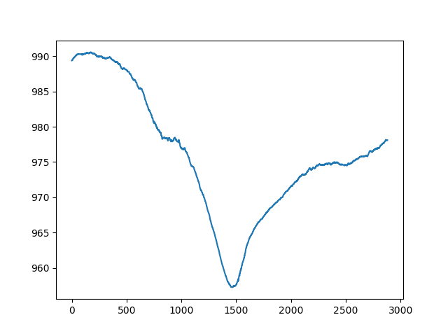
We can see how the pressure drops significantly as the storm passes over the weather station. However, the plot could be improved with some lables on the axes, and a title. To add them to the figure, change our script to include the following:
import pandas as pd
import matplotlib.pyplot as plt

data = pd.read_csv('StormEleanor_2_3_Jan.csv', delimiter=',', header=0)

pressure_data = data['Pair_Avg']

plt.plot(pressure_data)
plt.ylabel("Pressure (hPa)")
plt.title("Average Pressure, JCMB Weather Station, 2-3rd Jan 2018")

# Hmmm, what about the time along the x axis?...
As you can see, adding labels is easy enough with the ylabel and title functions. But although there is an xlabel function, our x data is simply integers for each timestep, rather than an actual timestamp. It would be more readable if we could convert these integers into actual times, and plot these instead. We can do this with the help of the datetime module, a built-in python module for dealing with dates and times.
# import the required libraries and modules
import datetime

# Code to create the timeseries values
date_time_series = []
date_time = datetime.datetime(2018, 1, 2)
date_at_end = datetime.datetime(2018, 1, 3, 23, 59)
step = datetime.timedelta(minutes=1)

while date_time <= date_at_end:
  date_time_series.append(date_time)
  date_time += step

print(date_time_series)
Let’s break this down:
- We add
datetimeto our import statements at the start of the script - We create an empty list to store our dates
- We set the first date in the series, which is Midnight (00:00) on the 2nd January 2018. (Midnight is set by default if no hours/minutes are specified)
- We set the end date for our date, which is 23:59 on the 3rd January 2018.
- Set the timestep as a
timedeltaobject. (Remember, the weather station data is recorded every minute. - Iterate by adding the time delta to the start time, and appending the new time step to the list, until we reach the final time.
Finally, we now have a new list of times that we can plot. When we call plt.plot() this time, we are going to supply two arguments: an x series (datetimes) and a y series (pressure).
Add the above code into your script after the data loading lines, then run the script again. (Make sure you still have a plt.savefig() call at the end).
We can also add a few extra matplotlib functions to tidy up our plot:
- (Optional) It will probably look nice if the x-labels are rotated slightly so that the times don’t overlap. We can do this by setting the
rotationargument in theplt.xticks()function. - To tidy up the axes, and scale them correctly, we can add a call to
plt.tight_layout()just before we save the figure.
The final script should look now look like this:
import pandas as pd
import matplotlib.pyplot as plt
import datetime

data = pd.read_csv('StormEleanor_2_3_Jan.csv', delimiter=',', header=0)

pressure_data = data['Pair_Avg']

date_time_series = []
date_time = datetime.datetime(2018, 1, 2)
date_at_end = datetime.datetime(2018, 1, 3, 23, 59)
step = datetime.timedelta(minutes=1)

while date_time <= date_at_end:
  date_time_series.append(date_time)
  date_time += step

plt.plot(date_time_series, pressure_data)
plt.ylabel("Pressure (hPa)")
plt.xlabel("Time")
plt.title("Average Pressure, JCMB Weather Station, 2-3rd Jan 2018")
plt.xticks(rotation=-60)
plt.tight_layout()
plt.savefig("pressure_final.png")
Make sure the script is saved, and then run it. Open up the “pressure_final.png” file to see your results.
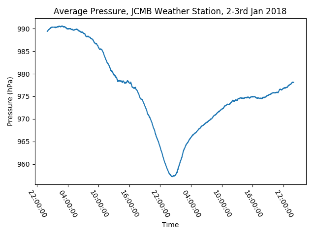
The final figure should look like this:
Summary
In this tutorial we have looked at why Python is popular for scientific programming, and gotten a feel for how Python looks and feels. Hopefully, you have learnt some of the basic syntax, and how to write and run simple python scripts to read in data from text files, and make a simple plot of some of the data.
Tutorial outcomes:
- You have a feel for how widely used Python is, and why it is popular
- You can run a simple test Python program on your computer
- You can read in data from a text file using the core Python language
- You can use modules and packages to streamline data reading and analysis
- You can make simple figures with matplotlib
- You have a feel for some of the basic syntax and data structures of Python