Tutorial aims:
- Learn base R syntax for data manipulation
- Turn messy data into tidy data with
tidyr - Use efficient tools from the
dplyrpackage to manipulate data
Steps:
- Subset, extract and modify data with R base operators
- What is tidy data, and how do we achieve it?
- Explore the most common and useful functions of
dplyr - Challenge yourself!
Data come in all sorts of different shapes and formats, and what is useful or practical for one application is not necessarily so for another. R has specific requirements about the setup and the types of data that can be passed to functions, so one of the best skills in your coding toolbox is being able to play with your data like putty and give it any shape you need!
This tutorial is an introduction to data manipulation and only requires an understanding of how to import and create objects in R. That said, there’s still a lot of content in here for a beginner, so do not hesitate to complete only the base R section in one session, and the dplyr section in another. (Remember! The beauty of a script is that you can pick up where you left off, anytime.)
Haven’t used R before, or need a refresher? No worries! Check out our Intro to R and RStudio tutorial, and then come back here to master tidy data management!
Know all of this already? Fast forward to our Efficient Data Manipulation tutorial for more advanced dplyr fun or to Advanced Data Manipulation tutorial for even deeper dplyr knowledge.
In this tutorial, we will start by showing some ways to manipulate data using base R syntax (without any extra package), because you will often see solutions online using this syntax, and it is good to understand how objects are built (and how to take them apart). After that, we will introduce principles of tidy data to encourage best practice in data collection and organisation. We will then start using packages from the Tidyverse , which is quickly becoming the norm in R data science, and offers a neater, clearer way of coding than using only base R functions.
All the files you need to complete this tutorial can be downloaded from this repository. Clone and download the repo as a zip file, then unzip it.
1. Subset, extract and modify data with R operators
Data frames are R objects made of rows and columns containing observations of different variables: you will often be importing your data that way. Sometimes, you might notice some mistakes after importing, need to rename a variable, or keep only a subset of the data that meets some conditions. Let’s dive right in and do that on the EmpetrumElongation.csv dataset that you have downloaded from the repository.
Create a new, blank script, and add in some information at the top, for instance the title of the tutorial, your name, and the date (remember to use hashtags # to comment and annotate your script).
This dataset represents annual increments in stem growth, measured on crowberry shrubs on a sand dune system. The Zone field corresponds to distinct zones going from closest (2) to farthest (7) from the sea.
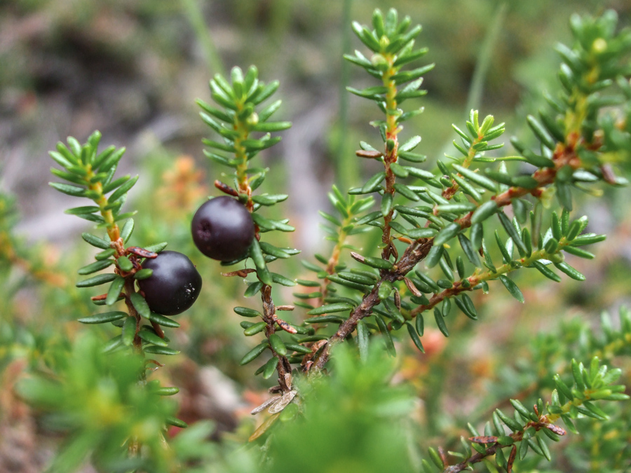 A crowberry shrub, Empetrum hermaphroditum. Isn’t it pretty?
We have seen in our intro tutorial that we can access variables in R by using the dollar sign $. This is already one way of subsetting, as it essentially reduces your data frame (2 dimensions) to a vector (1 dimension). You can also access parts of a data frame using square brackets [ , ]. The first number you put will get the row number, and the second the column. Leave one blank to keep all rows or all columns.
# Set your working directory to where the folder is saved on your computer
setwd("file-path")

# Load the elongation data
elongation <- read.csv("EmpetrumElongation.csv", header = TRUE)

# Check import and preview data
head(elongation)   # first few observations
str(elongation)    # types of variables

# Let's get some information out of this object!
elongation$Indiv   # prints out all the ID codes in the dataset
length(unique(elongation$Indiv))   # returns the number of distinct shrubs in the data

# Here's how we get the value in the second row and fifth column
elongation[2,5]

# Here's how we get all the info for row number 6
elongation[6, ]

# And of course you can mix it all together!
elongation[6, ]$Indiv   # returns the value in the column Indiv for the sixth observation
# (much easier calling columns by their names than figuring out where they are!)
Subsetting with brackets using row and column numbers can be quite tedious if you have a large dataset and you don’t know where the observations you’re looking for are situated! And it’s never recommended anyway, because if you hard-code a number in your script and you add some rows later on, you might not be selecting the same observations anymore! That’s why we can use logical operations to access specific parts of the data that match our specification.
# Let's access the values for Individual number 603
elongation[elongation$Indiv == 603, ]
There’s a lot to unpack here! We’re saying: “Take this dataframe (elongation), subset it ([ , ]) so as to keep the rows (writing the expression on the left-hand of the comma) for which the value in the column Indiv ($Indiv) is exactly (==) 603”. Note: The logical expression works here because the Indiv column contains numeric values: to access data that is of character or factor type, you would use quotation marks: elongation$Indiv == "six-hundred-and-three".
Operators for logical operations
Here are some of the most commonly used operators to manipulate data. When you use them to create a subsetting condition, R will evaluate the expression, and return only the observations for which the condition is met.
==: equals exactly
<, <=: is smaller than, is smaller than or equal to
>, >=: is bigger than, is bigger than or equal to
!=: not equal to
%in%: belongs to one of the following (usually followed by a vector of possible values)
&: AND operator, allows you to chain two conditions which must both be met
|: OR operator, to chains two conditions when at least one should be met
!: NOT operator, to specify things that should be omitted
Let’s see them in action!
# Subsetting with one condition

elongation[elongation$Zone < 4, ]    # returns only the data for zones 2-3
elongation[elongation$Zone <= 4, ]   # returns only the data for zones 2-3-4


# This is completely equivalent to the last statement
elongation[!elongation$Zone >= 5, ]   # the ! means exclude


# Subsetting with two conditions
elongation[elongation$Zone == 2 | elongation$Zone == 7, ]    # returns only data for zones 2 and 7
elongation[elongation$Zone == 2 & elongation$Indiv %in% c(300:400), ]    # returns data for shrubs in zone 2 whose ID numbers are between 300 and 400
As you can see, the more demanding you are with your conditions, the more cluttered the code becomes. We will soon learn some functions that perform these actions in a cleaner, more minimalist way, but sometimes you won’t be able to escape using base R (especially when dealing with non-data-frame objects), so it’s good to understand these notations.
Did you notice that last bit of code: c(300:400) ? We saw in our intro tutorial that we can use c() to concatenate elements in a vector. Using a colon between the two numbers means counting up from 300 to 400.
Other useful vector sequence builders are:
seq() to create a sequence, incrementing by any specified amount. E.g. try seq(300, 400, 10)
rep() to create repetitions of elements. E.g. rep(c(1,2), 3) will give 1 2 1 2 1 2.
You can mix and match! What would rep(seq(0, 30, 10), 4)give?
And finally, let’s say you need to modify some values or factor levels, or want to create a new column? Now that you know how to access parts of a dataframe, you can do all of that. You only need an extra tool: the assign arrow <- to overwrite data.
Creating and overwriting objects
Remember how we’ve been using the arrow <- to create new objects? This is a special convention in R that allows you to pick whichever name you want and assign it to an object (vector, list, data frame…).
Something to keep in mind is that if you use a name again in a same session, it will overwrite the former object. With experience, you can start making changes to an object and overwrite as you go, to “update” the object rather than creating many intermediaries (“object1”, “object2”, …). However, when you’re starting out, it’s a good idea to create these intermediary objects, or at least to create a “working copy” that you can reassign to the main data object once you’re satisfied with the changes.
As you will now see, we can also make use of the arrow <- to overwrite specific values or range of values we need to change.
## CHANGING VARIABLE NAMES AND VALUES IN A DATA FRAME

# Let's create a working copy of our object
elong2 <- elongation

# Now suppose you want to change the name of a column: you can use the names() function
# Used on its own, it returns a vector of the names of the columns. Used on the left side of the assign arrow, it overwrites all or some of the names to value(s) of your choice.

names(elong2)                 # returns the names of the columns

names(elong2)[1] <- "zone"    # Changing Zone to zone: we call the 1st element of the names vector using brackets, and assign it a new value
names(elong2)[2] <- "ID"      # Changing Indiv to ID: we call the 2nd element and assign it the desired value

# Now suppose there's a mistake in the data, and the value 5.1 for individual 373 in year 2008 should really be 5.7

## - option 1: you can use row and column number
elong2[1,4] <- 5.7

## - option 2: you can use logical conditions for more control
elong2[elong2$ID == 373, ]$X2008 <- 5.7   # completely equivalent to option 1
Can you spot pros and cons of options 1 and 2 above?
Option 1 is compact, but requires you to know exactly where the value to be corrected is. If you reimport your dataset at a later time with new values, it may not be in the same place.
Option 2 is longer and more difficult to read (it uses brackets to extracts the row corresponding to individual #373, and then the dollar sign to access just the column called X2008), but provides fine control, and the code will run even if the observation moves in your dataset.
Using the same techniques, you can specify variable classes, which will be highly useful when we get to designing statistical models and need grouping variables like factors.
## CREATING A FACTOR

# Let's check the classes
str(elong2)

# The zone column shows as integer data (whole numbers), but it's really a grouping factor (the zones could have been called A, B, C, etc.) Let's turn it into a factor:

elong2$zone <- as.factor(elong2$zone)        # converting and overwriting original class
str(elong2)                                  # now zone is a factor with 6 levels
And what if you’re not happy with the factor levels? You can see the names of the factors with the levels() function… and yes, overwrite them, too.
## CHANGING A FACTOR'S LEVELS

levels(elong2$zone)  # shows the different factor levels

levels(elong2$zone) <- c("A", "B", "C", "D", "E", "F")   # you can overwrite the original levels with new names

# You must make sure that you have a vector the same length as the number of factors, and pay attention to the order in which they appear!
That was a lot, but now you’ll be able to adapt these little chunks of code to manipulate your own data. The next sections will hopefully make things even easier, as they’ll teach you more intuitive functions to accomplish the same things.
2. What is tidy data, and how do we achieve it?
The way you record information in the field or in the lab is probably very different to the way you want your data entered into R. In the field, you want tables that you can ideally draw up ahead of time and fill in as you go, and you will be adding notes and all sorts of information in addition to the data you want to analyse. For instance, if you monitor the height of seedlings during a factorial experiment using warming and fertilisation treatments, you might record your data like this:
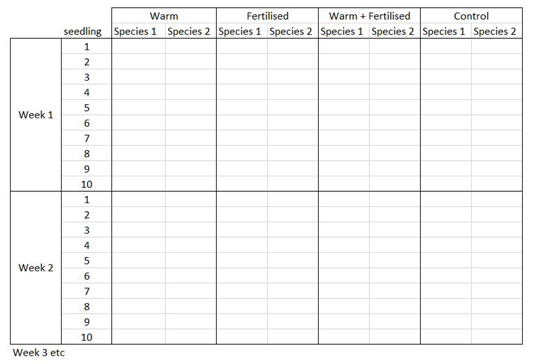
Let’s say you want to run a test to determine whether warming and/or fertilisation affected seedling growth. You may know how your experiment is set up, but R doesn’t! At the moment, with 8 measures per row (combination of all treatments and species for one replicate, or block), you cannot run an analysis. On the contrary, tidy datasets are arranged so that each row represents an observation and each column represents a variable. In our case, this would look something like this:
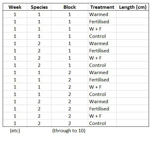
This makes a much longer dataframe row-wise, which is why this form is often called long format. Now if you wanted to compare between groups, treatments, species, etc., R would be able to split the dataframe correctly, as each grouping factor has its own column.
Based on this, do you notice something not quite tidy with our previous object elongation? We have observation of the same variable, i.e. stem length, spread across multiple columns representing different years.
The gather() function from the tidyr package will let us convert this wide-format table to a tidy dataframe. We want to create a single column Year that will have years currently in the columns (2007-2012) repeated for each individual. From this, you should be able to work out that the dataframe will be six times longer than the original. We also want a column Length where all the growth data associated to each year and individual will go.
Note: This function is slightly unusual as you are making up your own column names in the second (key) and third (value) arguments, rather than passing them pre-defined objects or values like most R functions. Here, year is our key and length is our value.
install.packages("tidyr")  # install the package
library(tidyr)             # load the package


elongation_long <- gather(elongation, Year, Length,                           # in this order: data frame, key, value
                          c(X2007, X2008, X2009, X2010, X2011, X2012))        # we need to specify which columns to gather

# Here we want the lengths (value) to be gathered by year (key)

# Let's reverse! spread() is the inverse function, allowing you to go from long to wide format
elongation_wide <- spread(elongation_long, Year, Length)
Notice how we used the column names to tell gather() which columns to reshape. This is handy if you only have a few, and if the columns change order eventually, the function will still work. However, if you have a dataset with columns for 100 genes, for instance, you might be better off specifying the column numbers:
elongation_long2 <- gather(elongation, Year, Length, c(3:8))
However, these functions have limitations and will not work on every data structure. To quote Hadley Wickham, “every messy dataset is messy in its own way”. This is why giving a bit of thought to your dataset structure before doing your digital entry can spare you a lot of frustration later!
Once you have the data in the right format, it’s much easier to analyse them and visualise the results. For example, if we want to find out if there is inter-annual variation in the growth of Empetrum hermaphroditum, we can quickly make a boxplot:
boxplot(Length ~ Year, data = elongation_long,
        xlab = "Year", ylab = "Elongation (cm)",
	main = "Annual growth of Empetrum hermaphroditum")
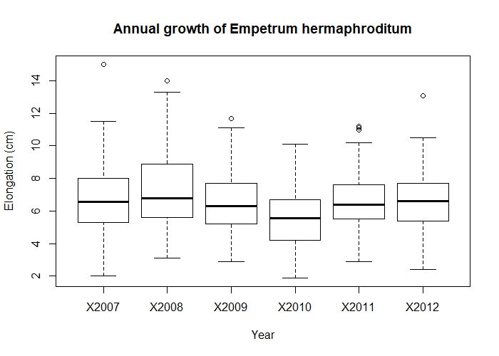 Annual growth of Empetrum hermaphroditum.
.
From looking at the boxplot, there is a fairly big overlap between the annual growth in each year - nothing special to see. (Don’t worry, we’ll learn to make much prettier and interesting graphs in our data visualisation tutorials.)
3. Explore the most common and useful functions of dplyr
The package dplyr is a fantastic bundle of intuitive functions for data manipulation, named after the action they perform. A big advantage of these functions is that they take your data frame as a first argument, so that you can refer to columns without explicitly having to refer to the full object (so you can drop those $ signs!). Let’s meet the most common and useful functions by working on the long format object we just created, elongation_long. First, install and load the package.
install.packages("dplyr")  # install the package
library(dplyr)              # load the package
3a. rename() variables
This lets you change the name(s) of a column or columns. The first argument is the data frame, the second (and third, etc.) takes the form New name = Old name.
elongation_long <- rename(elongation_long, zone = Zone, indiv = Indiv, year = Year, length = Length)     # changes the names of the columns (getting rid of capital letters) and overwriting our data frame

# As we saw earlier, the base R equivalent would have been
names(elongation_long) <- c("zone", "indiv", "year", "length")
3b. filter() rows and select()columns
These are some of the most routine functions that let you reduce your data frame to just the rows and columns you need. The filter() function works great for subsetting rows with logical operations. The select() function lets you specify which columns to keep. Note: the select() function often clashes with functions of the same name in other packages, and for that reason it is recommended to always use the notation dplyr::select() when calling it.
# FILTER OBSERVATIONS

# Let's keep observations from zones 2 and 3 only, and from years 2009 to 2011

elong_subset <- filter(elongation_long, zone %in% c(2, 3), year %in% c("X2009", "X2010", "X2011")) # you can use multiple different conditions separated by commas

# For comparison, the base R equivalent would be (not assigned to an object here):
elongation_long[elongation_long$zone %in% c(2,3) & elongation_long$year %in% c("X2009", "X2010", "X2011"), ]
Note that here, we use %in% as a logical operator because we are looking to match a list of exact (character) values. If you want to keep observations within a range of numeric values, you either need two logical statements in your filter() function, e.g. length > 4 & length <= 6.5 or you can use the convenient between() function, e.g. between(length, 4, 6.5).
See how dplyris already starting to shine by avoiding repetition and calling directly the column names without needing to call the object every time?
To quote or not to quote?
You may have noticed how we sometimes call values in quotes "", and sometimes not. This depends on:
- Whether the value you are calling is a character or numeric value: above,
zoneis of class integer (a number), so we don’t need quotes around the values it takes, butyearis a character (letters), so needs them. - Whether you are calling an existing object or referring to a value that R does not yet know about. Compare:
new.object <- elongation_longandnew.object <- "elongation_long"
The first creates a duplicate of our object, because R recognises the name as an object in our environment. In the second case, you’re creating an object consisting of one character value.
It takes time and practice to get used to these conventions, but just keep an eye out for error messages and you’ll get there.
Now that we know how to subset rows, let’s do the same with columns!
# SELECT COLUMNS

# Let's ditch the zone column just as an example

elong_no.zone <- dplyr::select(elongation_long, indiv, year, length)   # or alternatively
elong_no.zone <- dplyr::select(elongation_long, -zone) # the minus sign removes the column

# For comparison, the base R equivalent would be (not assigned to an object here):
elongation_long[ , -1]  # removes first column

# A nice hack! select() lets you rename and reorder columns on the fly
elong_no.zone <- dplyr::select(elongation_long, Year = year, Shrub.ID = indiv, Growth = length)

# Neat, uh?
3c. mutate() your dataset by creating new columns
Something we have not yet touched on is how to create a new column. This is useful when you want to perform an operation on multiple columns, or perhaps reclassify a factor. The mutate() function does just that, and also lets you define the name of the column. Here let’s use our old wide-format object elongation and create a column representing total growth for the period 2007-2012:
# CREATE A NEW COLUMN

elong_total <- mutate(elongation, total.growth = X2007 + X2008 + X2009 + X2010 + X2011 + X2012)
Now, let’s see how we could accomplish the same thing on our long-format data elongation_long by using two functions that pair extremely well together: group_by() and summarise().
3d. group_by() certain factors to perform operations on chunks of data
The most important thing to understand about this function is that you don’t see any visible change to your data frame. It creates an internal grouping structure, which means that every subsequent function you run on it will use these groups, and not the whole dataset, as an input. It’s very useful when you want to compute summary statistics for different sites, treatments, species, etc.
# GROUP DATA

elong_grouped <- group_by(elongation_long, indiv)   # grouping our dataset by individual
Compare elong_grouped and elongation_long : they should look exactly the same. But now, let’s use summarise() to calculate total growth of each individual over the years.
3e. summarise() data with a range of summary statistics
This function will always aggregate your original data frame, i.e. the output data frame will be shorter than the input. Here, let’s contrast summing growth increments over the study period on the original dataset vs our new grouped dataset.
# SUMMARISING OUR DATA

summary1 <- summarise(elongation_long, total.growth = sum(length))
summary2 <- summarise(elong_grouped, total.growth = sum(length))
The first summary corresponds to the sum of all growth increments in the dataset (all individuals and years). The second one gives us a breakdown of total growth per individual, our grouping variable. Amazing! We can compute all sorts of summary statistics, too, like the mean or standard deviation of growth across years:
summary3 <- summarise(elong_grouped, total.growth = sum(length),
                                     mean.growth = mean(length),
                                     sd.growth = sd(length))
Less amazing is that we lose all the other columns not specified at the grouping stage or in a summary operation. For instance, we lost the column year because there are 5 years for each individual, and we’re summarising to get one single growth value per individual. Always create a new object for summarised data, so that your full dataset doesn’t go away! You can always merge back some information at a later stage, like we will see now.
6. ..._join() datasets based on shared attributes
Sometimes you have multiple data files concerning a same project: one for measurements taken at various sites, others with climate data at these sites, and perhaps some metadata about your experiment. Depending on your analytical needs, it may be very useful to have all the information in one table. This is where merging, or joining, datasets comes in handy.
Let’s imagine that the growth data we have been working with actually comes from an experiment where some plants where warmed with portable greenhouses (W), others were fertilised (F), some received both treatments (WF) and some were control plants (C). We will import this data from the file EmpetrumTreatments.csv, which contains the details of which individuals received which treatments, and join it with our main dataset elongation_long. We can do this because both datasets have a column representing the ID of each plant: this is what we will merge by.
There are many types of joins you can perform, which will make sense to you if you are familiar with the SQL language. They differ in how they handle data that is not shared by both tables, so always ask yourself which observations you need to keep and which you want to drop, and look up the help pages if necessary (in doubt, full_join() will keep everything). In the following example, we want to keep all the information in elong_long and have the treatment code repeated for the five occurrences of every individual, so we will use left_join().
# Load the treatments associated with each individual

treatments <- read.csv("EmpetrumTreatments.csv", header = TRUE, sep = ";")
head(treatments)

# Join the two data frames by ID code. The column names are spelled differently, so we need to tell the function which columns represent a match. We have two columns that contain the same information in both datasets: zone and individual ID.

experiment <- left_join(elongation_long, treatments, by = c("indiv" = "Indiv", "zone" = "Zone"))

# We see that the new object has the same length as our first data frame, which is what we want. And the treatments corresponding to each plant have been added!
If the columns to match have the exact same name, you can omit them as they are usually automatically detected. However, it is good practice to specify the merging condition, as it ensures more control over the function. The equivalent base R function is merge() and actually works very well, too:
experiment2 <- merge(elongation_long, treatments, by.x = c("zone", "indiv"), by.y = c("Zone", "Indiv"))
# same result!
Now that we have gone to the trouble of adding treatments into our data, let’s check if they affect growth by drawing another box plot.
boxplot(length ~ Treatment, data = experiment)
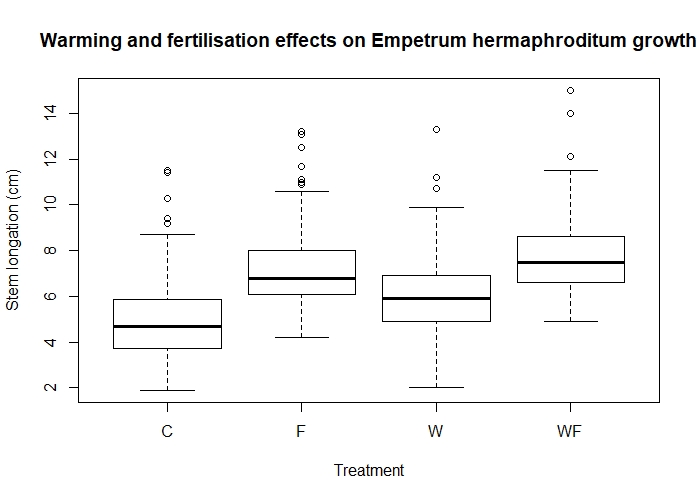 Effects of warming (W) and fertilisation (F) treatments on crowberry growth (fictional data!).
Are these differences statistically significant? We’ll find out how to test this in our modelling tutorial!
But for now, don’t you think it’s enough for one tutorial? Congratulations for powering through and getting this far! If you want to test your knowledge, try your hand at the data manipulation challenge below.
Challenge yourself!
Let’s see if you can apply some of the functions we have learned today in a different context. In the repository, you will find the file dragons.csv, which gives the length (in cm) of the fire plumes breathed by dragons of different species when fed different spices.
Your challenge is to make the data tidy (long format) and to create a boxplot for each species showing the effect of the spices on plume size, so you can answer the questions: Which spice triggers the most fiery reaction? And the least?
However, you find out that your field assistant was a bit careless during data collection, and let slip many mistakes which you will need to correct.
- The fourth treatment wasn’t paprika at all, it was turmeric.
- There was a calibration error with the measuring device for the tabasco trial, but only for the Hungarian Horntail species. All measurements are 30 cm higher than they should be.
- The lengths are given in centimeters, but really it would make sense to convert them to meters.
Now let’s see what you can do!
Stuck? Click for a few hints
- Struggling to rename the paprika column? Think about the handy
rename()function! - There are many ways to correct a selection of values, but they will all involve accessing these specific data by combining conditional statements about the treatment/column (tabasco) and the species (horntail). You could store the correct values in a vector, and overwrite the old values by using appropriate subsetting. (Tip: arithmetic operations on a vector are applied to each element individually, so that
c(1, 2, 3) + 1returns2, 3, 4.) - The
mutate()function lets you create a new column that can be based on existing columns. Ideal for things like converting units… It may be wise to have all the plume lengths in one column (long, or tidy format), before using this. - Struggling to reshape the dataset? Remember that you are trying to
gather()the plume observations (value) by treatment, in this case spice (key).
Click to see the solution
Here is a solution to clean the data and achieve the boxplots.
## Load data

dragons <- read.csv('dragons.csv', header = TRUE)


## Clean the dataset

# Change paprika to turmeric

dragons <- rename(dragons, turmeric = paprika)


# Fix the calibration error for tabasco by horntail

correct.values  <- dragons$tabasco[dragons$species == 'hungarian_horntail'] - 30   # create a vector of corrected values

dragons[dragons$species == 'hungarian_horntail', 'tabasco'] <- correct.values      # overwrite the values in the dragons object
Here, it might have been simpler to change these values after reshaping the data to long format. You might also have used a dplyr solution. There are many ways to achieve a same result in R! In the next data manipulation tutorial, we will learn more ways to recode variables or change many values at once. As a taster, a neat way to do the above would be to use dplyr’s mutate() function along with the logical function ifelse() to conditionally change only these values:
dragons.2 <- mutate(dragons, tabasco = ifelse(species == 'hungarian_horntail', tabasco - 30, tabasco))

# This creates (overwrites) the column tabasco using the following logic: if the species is Hungarian Horntail, deduct 30 from the values in the (original) tabasco column; if the species is NOT horntail (i.e. all other species), write the original values.
But whatever works for you! Now let’s finish cleaning the dataset and make those plots:
# Reshape the data from wide to long format

dragons_long <- gather(dragons, key = 'spice', value = 'plume', c('tabasco', 'jalapeno', 'wasabi', 'turmeric'))


# Convert the data into meters

dragons_long <- mutate(dragons_long, plume.m = plume/100)    # Creating a new column turning cm into m


# Create a subset for each species to make boxplots

horntail <- filter(dragons_long, species == 'hungarian_horntail')            # the dplyr way of filtering
green <- filter(dragons_long, species == 'welsh_green')
shortsnout <- dragons_long[dragons_long$species == 'swedish_shortsnout', ]   # maybe you opted for a base R solution instead?


# Make the boxplots

par(mfrow=c(1, 3))      # you need not have used this, but it splits your plotting device into 3 columns where the plots will appear, so all the plots will be side by side.

   boxplot(plume.m ~ spice, data = horntail,
           xlab = 'Spice', ylab = 'Length of fire plume (m)',
           main = 'Hungarian Horntail')


   boxplot(plume.m ~ spice, data = green,
           xlab = 'Spice', ylab = 'Length of fire plume (m)',
           main = 'Welsh Green')


   boxplot(plume.m ~ spice, data = shortsnout,
           xlab = 'Spice', ylab = 'Length of fire plume (m)',
           main = 'Swedish Shortsnout')
So there you are! Did your plots look something like this?
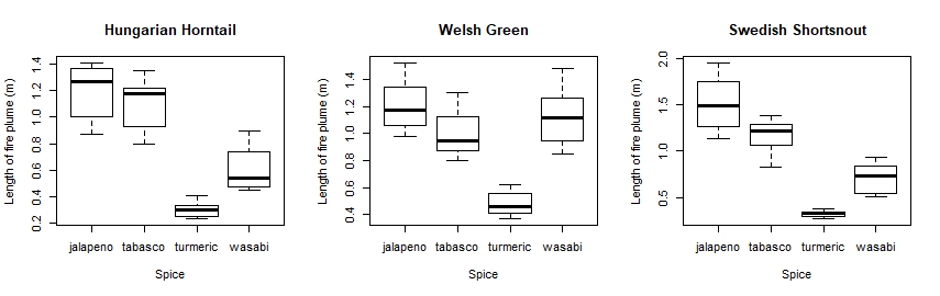
It looks like jalapeños are proper dragon fuel, but turmeric not so much!
Tutorial Outcomes:
- You can use
$and[]operators to subset elements of data frames in the classic R notation - You understand the format required for analyses in R, and can use the package
tidyrto achieve it. - You can manipulate, subset, create and merge data with
dplyr
When you’re ready for more dplyr tips and workflows, follow up with our Efficient data manipulation tutorial!
Doing this tutorial as part of our Data Science for Ecologists and Environmental Scientists online course?
This tutorial is part of the Stats from Scratch stream from our online course. Go to the stream page to find out about the other tutorials part of this stream!
If you have already signed up for our course and you are ready to take the quiz, go to our quiz centre. Note that you need to sign up first before you can take the quiz. If you haven't heard about the course before and want to learn more about it, check out the course page.