Tutorial aims:
- Understand what are R and R Studio
- Develop the good habit of working with scripts
- Learn to import data in R
- Learn to manipulate R objects like vectors and data frames
- Make a simple plot
Steps:
- Download R and RStudio
- Import and check data
- Calculate species richness
- Create a vector and plot it
- Create a data frame and plot it
- Challenge yourself
- Glossary
In our first tutorial we will begin to explore “R” as a tool to analyse and visualise data.
What is R?
R is a statistical programming language that has rapidly gained popularity in many scientific fields. It was developed by Ross Ihaka and Robert Gentleman as an open source implementation of the “S” programming language. (Next time you need a fun fact, you can say “Did you know that S came before R?”) R is also the name of the software that uses this language for statistical computing. With a huge online support community and dedicated packages that provide extra functionality for virtually any application and field of study, there’s hardly anything you can’t do in R.
If you already know your way around statistical softwares like Minitab or SPSS, the main difference is that R has no graphical user interface, which means there are no buttons to click and no dropdown menus. R can be run entirely by typing commands into a text interface (welcome to the Matrix!). This may seem a little daunting, but it also means a whole lot more flexibility, as you are not relying on a pre-determined toolkit for your analyses.
Thanks for joining us on your learning journey. Like with any language, there is a learning curve (trust me, I’m learning German at the moment), but we will take it step by step, and in no time you will be coding your own analyses and graphs!
If you need any more convincing, why are we using R and not one of the many other statistical packages like MATLAB, Minitab, or even Microsoft Excel? Well, R is great because:
- R is free and open source, and always will be! Anybody can use the code and see exactly how it works.
- Because R is a programming language rather than a graphical interface, the user can easily save scripts as small text files for use in the future, or share them with collaborators.
- R has a very active and helpful online community - normally a quick search is all it takes to find that somebody has already solved the problem you’re having. You can start with our page with useful links!
1. Download R and RStudio
As we said before, R itself does not have a graphical interface, but most people interact with R through graphical platforms that provide extra functionality. We will be using a program called RStudio as a graphical front-end to R, so that we can access our scripts and data, find help, and preview plots and outputs all in one place.
You can download R from CRAN (The Comprehensive R Archive Network). Select the link appropriate for your operating system.
Then, download RStudio from the RStudio website (select the free open source desktop version).
If you are using a Mac, in addition to R and RStudio, you need to download XQuartz (available here).
Open RStudio. Click on “File/New File/R script”.
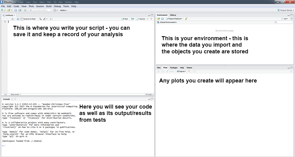
You will now see a window like the one above. You can type code directly into the console on the lower left (doesn’t mean that you should*!). Pressing enter at the end of the line runs the code (try typing 2 + 2 and running it now). You can (should!) also write your code in the script file in the top left window. To run a line of code from your script, press Ctrl+R on Windows or Cmd+Enter on a Mac. On newer Windows computers, the default shortcut is Ctrl+Enter. The environment window gives you an overview of your current workspace**. You will see the data you have imported, objects you have created, functions you have defined, etc. Finally, the last panel has multiple tabs and will preview your plot and allow you to navigate around folders and look at the packages you currently have installed and loaded.
*A note about scripts (We love scripts!): Remember that if you enter code directly into the console, it will not be saved by R: it runs and disappears (although you can access your last few operations by hitting the ‘up’ key on your keyboard). Instead, by typing your code into a script file, you are creating a reproducible record of your analysis. Writing your code in a script is similar to writing an essay in Word: it saves your progress and you can always pick up where you left off, or make some changes to it. (Remember to click Save (Ctrl+S) often, so that you actually save your script!)
When writing a script, it’s useful to add comments to describe what you are doing by inserting a hasthag # in front of a line of text. R will see anything that begins with #as text instead of code, so it will not try to run it, but the text will provide valuable information about the code for whoever is reading your script (including future you!). Like with any piece of writing, scripts benefit from structure and clarity: we will learn more about proper coding etiquette in a later tutorial.
**A quicker note about the workspace: The workspace will have everything you have used in a session floating around your computer memory. When you exit, R will ask you if you want to save the current workspace. You almost never need to, and it’s best to click no and start with a clear slate every time. (DO make sure you save your script though!!)
Begin to write in your script
For now, start by recording who is writing, the date, and the main goal - in our case, determining how many species from different taxa have been recorded in Edinburgh. Here’s an example, which you can copy, paste and edit into your new script:
# Coding Club Workshop 1 - R Basics
# Learning how to import and explore data, and make graphs about Edinburgh's biodiversity
# Written by Gergana Daskalova 06/11/2016 University of Edinburgh
The next few lines of code usually load the packages you will be needing for your analysis. A package is a bundle of commands that can be loaded into R to provide extra functionality. For example, you might load a package for formatting data, or for making maps. (Or for making graphs with cats on them, or whatever floats your boat… As we said before, there’s virtually nothing you cannot do!)
To install a package, type install.packages("package-name"). You only need to install packages once, so in this case you can type directly in the console box, rather than saving the line in your script and re-installing the package every time.
Once installed, you just need to load the packages using library(package-name). Today we will be using the dplyr package to provide extra commands for formatting and manipulating data. (You will learn more about the powerful features of dplyr in a later tutorial).
The next lines of code should define your working directory. This is a folder on your computer where R will look for data, save your plots, etc. To make your workflow easier, it is good practice to save everything related to one project in the same place, as it will save you a lot of time typing up computer paths or hunting for files that got saved R-knows-where. For instance, you could save your script and all the data for this tutorial in a folder called “Intro_to_R”. (It is good practice to avoid spaces in file names as it can sometimes confuse R.) For bigger projects, consider having a root folder with the name of the project (e.g. “My_PhD”) as your working directory, and other folders nested within to separate data, scripts, images, etc. (e.g. My_PhD/Chapter_1/data, My_PhD/Chapter_1/plots, My_PhD/Chapter_2/data, etc.)
To find out where your working directory is now, run the code getwd(). If you want to change it, you can use setwd(). Set your working directory to the folder you just downloaded from GitHub:
install.packages("dplyr")
library(dplyr)
# Note that there are quotation marks when installing a package, but not when loading it
# and remember that hashtags let you add useful notes to your code!

setwd("C:/User/CC-1-RBasics-master")
# This is an example filepath, alter to your own filepath
Watch out! Note that on a Windows computer, a copied-and-pasted file path will have backslashes separating the folders ("C:\folder\data"), but the filepath you enter into R should use forward slashes ("C:/folder/data").
2. Import and check data
Practice is the best way to learn any new language, so let’s jump straight in and do some of our own statistical analysis using a publicly available dataset of occurrence records for many animal, plant and fungi species. We downloaded the records for 2000-2016 (from the NBN Gateway ) and saved them as edidiv.csv. First, you will need to download the data.
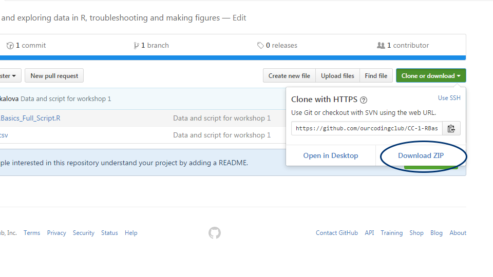
Follow the link, click on “Download Zip”, and save and unzip the folder somewhere on your computer. (Never heard of Github? Don’t worry, we will cover it in a later tutorial. For now, it’s simply the website where you can download our course material from.)
You can find all the files needed to complete this tutorial in this Github repository.
Click on Code and then Download zip. Remember to unzip the files before you start working with them in RStudio.
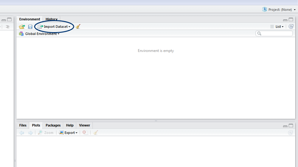
Now that you have the data saved on your computer, let’s import it! In RStudio, you can either click on the Import dataset button and navigate to where you have saved your file, or use the read.csv() command. If you use the button, a window will pop up previewing your data. Make sure that next to Heading you have selected Yes (this tells R to treat the first row of your data as the column names) and click Import. In the console, you will see the code for your import, which includes the file path - it’s a good idea to copy this code into your script, so that for future reference you know where your dataset came from.
R works best with .csv (comma separated values) files. If you entered your data in Excel, you would need to click on Save as and select csv as the file extension. When entering data in Excel, don’t put any spaces in your row names, as they will confuse R later (e.g. go for something like height_meters rather than height (m). Some computers save .csv files with semicolons ;, not commas , as the separators. This usually happens when English is not the first or only language on your computer. If your files are separated by semicolons, use read.csv2 instead of read.csv, or alternatively use the argument “sep” (for separator) in the read.csvfunction: r.csv("your-file-path", sep = ";").
edidiv <- read.csv("C:/Users/user/Desktop/Intro_to_R/edidiv.csv") # This is the file path based on where I saved the data, your filepath will be different
Remember to save your script once in a while! If you haven’t saved it already, why not save it in the same directory as the rest of the tutorial file, and give it a meaningful name.
A note about objects: R is an object-based language - this means that the data you import, and any values you create later, are stored in objects that you name. The arrow <- in the code above is how you assign objects. Here, we assigned our csv file to the object edidiv. We could just as easily have called it mydata or hello or biodiversity_recorded_around_Edinburgh_Scotland, but it’s best to choose a unique, informative, and short name. In the top right window of RStudio, you can see the names of any objects currently loaded into R. See your edidiv object?
When you import your data into R, it will most likely become an object called a data frame. A data frame is like a table, or spreadsheet - it has rows and columns with the different variables and observations you have loaded. But more on that later!
A really important step is to check that your data was imported without any mistakes. It’s good practice to always run this code and check the output in the console - do you see any missing values, do the numbers/names make sense? If you go straight into analysis, you risk later finding out that R didn’t read your data correctly and having to re-do it, or worse, analysing wrong data without noticing. To preview more than just the few first lines, you can also click on the object in your Environment panel, and it will show up as a spreadsheet in a new tab next to your open script. Large files may not display entirely, so keep in mind you could be missing rows or columns.
head(edidiv)                # Displays the first few rows
tail(edidiv)                # Displays the last rows
str(edidiv)                 # Tells you whether the variables are continuous, integers, categorical or characters
str(object.name) is a great command that shows the structure of your data. So often, analyses in R go wrong because R decides that a variable is a certain type of data that it is not. For instance, you might have four study groups that you simply called “1, 2, 3, 4”, and while you know that it should be a categorical grouping variable (i.e. a factor), R might decide that this column contains numeric (numbers) or integer (whole number) data. If your study groups were called “one, two, three, four”, R might decide it’s a character variable (words or strings of words), which will not get you far if you want to compare means among groups. Bottom line: always check your data structure!
You’ll notice the taxonGroup variable shows as a character variable, but it should be a factor (categorical variable), so we’ll force it to be one. When you want to access just one column of a data frame, you append the variable name to the object name with a dollar $sign. This syntax lets you see, modify, and/or reassign this variable.
head(edidiv$taxonGroup)     # Displays the first few rows of this column only
class(edidiv$taxonGroup)    # Tells you what type of variable we're dealing with: it's character now but we want it to be a factor

edidiv$taxonGroup <- as.factor(edidiv$taxonGroup)     # What are we doing here?!
In that last line of code, the as.factor() function turns whatever values you put inside into a factor (here, we specified we wanted to transform the character values in the taxonGroup column from the edidiv object). However, if you were to run just the bit of code on the right side of the arrow, it would work that one time, but would not modify the data stored in the object. By assigning with the arrow the output of the function to the variable, the original edidiv$taxonGroup in fact gets overwritten : the transformation is stored in the object. Try again to run class(edidiv$taxonGroup) - what do you notice?
# More exploration
dim(edidiv)                 # Displays number of rows and columns
summary(edidiv)             # Gives you a summary of the data
summary(edidiv$taxonGroup)  # Gives you a summary of that particular variable (column) in your dataset
3. Calculate species richness
Our edidiv object has occurrence records of various species collected in Edinburgh from 2000 to 2016. To explore Edinburgh’s biodiversity, we will create a graph showing how many species were recorded in each taxonomic group. You could calculate species richness in Excel, but that has several disadvantages, especially when working with large datasets like ours - you have no record of what you clicked on, how you sorted the data and what you copied/deleted - mistakes can slip by without you noticing. In R, on the other hand, you have your script, so you can go back and check all the steps in your analysis.
Species richness is simply the total number of different species in a given place or group. To know how many bird, plant, mammal, etc. species we have in Edinburgh, we first need to split edidiv into multiple objects, each containing rows for only one taxonomic group. We do this with the useful filter()function from the dplyrpackage.
Beetle <- filter(edidiv, taxonGroup == "Beetle")
# The first argument of the function is the data frame, the second argument is the condition you want to filter on. Because we only want the beetles here, we say: the variable taxonGroup MUST BE EXACTLY (==) Beetle - drop everything else from the dataset. (R is case-sensitive so it's important to watch your spelling! "beetle" or "Beetles" would not have worked here.)

Bird <- filter(edidiv, taxonGroup == "Bird")   # We do the same with birds. It's very similar to filtering in Excel if you are used to it.
# You can create the objects for the remaining taxa. If you need to remind yourself of the names and spellings, type summary(edidiv$taxonGroup)
You need to do these steps for ALL of the taxa in the data, here we have given examples for the first two. If you see an error saying R can’t find the object Beetle or similar, chances are you either haven’t installed and/or loaded the dplyr package. Go back and install it using install.packages("dplyr") and then load it using library(dplyr).
Once you have created objects for each taxon, we can calculate species richness, i.e. the number of different species in each group. For this, we will nest two functions together: unique(), which identifies different species, and length(), which counts them. You can try them separately in the console and see what they return!
a <- length(unique(Beetle$taxonName))
b <- length(unique(Bird$taxonName))
# You can choose whatever names you want for your objects, here I used a, b, c, d... for the sake of brevity.
If you type a (or however you named your count variables) in the console, what does it return? What does it mean? It should represent the number of distinct beetle species in the record.
Again, calculate species richness for the other taxa in the dataset. You’re probably noticing this is quite repetitive and using a lot of copying and pasting! That’s not particularly efficient - in future tutorials we will learn how to use more of dplyr’s functions and achieve the same result with way less code! You will be able to do everything you just did in ONE line (promise!).
4. Create a vector and plot it
Now that we have species richness for each taxon, we can combine all those values in a vector. A vector is another type of R object that stores values. As opposed to a data frame, which has two dimensions (rows and columns), a vector only has one. When you call a column of a data frame like we did earlier with edidiv$taxonGroup, you are essentially producing a vector - but you can also create them from scratch.
We do this using the c() function (c stands for concatenate, or chain if that makes it easier to remember). We can also add labels with the names()function, so that the values are not coming out of the blue.
biodiv <- c(a,b,c,d,e,f,g,h,i,j,k)     # We are chaining together all the values; pay attention to the object names you have calculated and their order
names(biodiv) <- c("Beetle",
                   "Bird",
                   "Butterfly",
                   "Dragonfly",
                   "Flowering.Plants",
                   "Fungus",
                   "Hymenopteran",
                   "Lichen",
                   "Liverwort",
                   "Mammal",
                   "Mollusc")
Notice:
- The spaces in front of and behind
<-and after,are added to make it easier to read the code. - All the labels have been indented on a new line - otherwise the line of code gets very long and hard to read.
- Take care to check that you are matching your vector values and labels correctly - you wouldn’t want to label the number of beetles as lichen species! The good thing about keeping a script is that we can go back and check that we have indeed assigned the number of beetle species to
a. Even better practice would have been to give more meaningful names to our objects, such asbeetle_sp,bird_sp, etc. - If you highlight a bracket
)with your mouse, R Studio will highlight its matching one in your code. Missing brackets, especially when you start nesting functions like we did earlier withlength(unique())are one of the most common sources of frustration and error when you start coding!
We can now visualise species richness with the barplot() function. Plots appear in the bottom right window in RStudio.
barplot(biodiv)
Ta-daaaa! But there are a few things not quite right that we should fix - there are no axis titles, not all column labels are visible, and the value for plant species (n = 521) exceeds the highest value on the y axis, so we need to extend it. The great thing about R is that you don’t need to come up with all the code on your own - you can use the help() function and see what arguments you need to add in. Look through the help output, what code do you need to add in?
help(barplot)     # For help with the barplot() function
help(par)         # For help with plotting in general
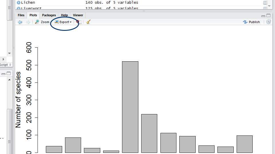
We also want to save our plot. To do this, click Export in the Plots window. If you don’t change the directory, the file will be saved in your working directory. You can adjust the dimensions to get the bar chart to look how you like it, and you should also add in a meaningful file name - Rplot01.png won’t be helpful when you try to find the file later.
You can also save your file by wrapping the code in the png() and dev.off() functions, which respectively open and shut down the plotting device.
png("barplot.png", width=1600, height=600)  # look up the help for this function: you can customise the size and resolution of the image
barplot(biodiv, xlab="Taxa", ylab="Number of species", ylim=c(0,600), cex.names= 1.5, cex.axis=1.5, cex.lab=1.5)
dev.off()
# The cex code increases the font size when greater than one (and decreases it when less than one).
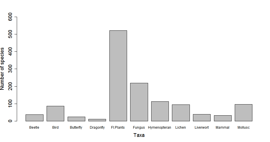 Figure 1. Species richness of several taxa in Edinburgh. Records are based on data from the NBN Gateway during the period 2000-2016.
5. Create a dataframe and plot it
In the last section we created vectors, i.e. a series of values, each with a label. This object type is suitable when dealing with just one set of values. Often, however, you will have more than one variable and have multiple data types - e.g. some continuous, some categorical. In those cases, we use data frame objects. Data frames are tables of values: they have a two-dimensional structure with rows and columns, where each column can have a different data type. For instance, a column called “Wingspan” would have numeric values measured on different birds (21.3, 182.1, 25.1, 8.9), and a column “Species” would have character values of with the names of the species (“House sparrow”, “Golden eagle”, “Eurasian kingfisher”, “Ruby-throated hummingbird”) Another possible data format is a matrix - a matrix can have several rows of data as well (e.g. you can combine vectors into a matrix), but the variables must be all of the same type. For instance they are all numerical and are the same length in terms of the number of rows.
A note on good housekeeping:
ALWAYS keep a copy of your raw data as you first collected it. The beauty of manipulating a file in an R script is that the modifications live on the script, not in the data. For Photoshop-savvy people, it’s like adding layers to an image: you’re not altering the original photo, just creating new things on top of it. That said, if you wrote a long piece of code to tidy up a large dataset and get it ready to analyse, you may not want to re-run the whole script every time you need to access the clean data. It’s therefore a good idea to save your shiny new object as a new csv file that you can load, ready-to-go, with just one command. We will now create a data frame with our species richness data, and then save it using write.csv().
We will use the data.frame() function, but first we will create an object that contains the names of all the taxa (one column) and another object with all the values for the species richness of each taxon (another column).
# Creating an object called "taxa" that contains all the taxa names
taxa <- c("Beetle",
          "Bird",
          "Butterfly",
          "Dragonfly",
          "Flowering.Plants",
          "Fungus",
          "Hymenopteran",
          "Lichen",
          "Liverwort",
          "Mammal",
          "Mollusc")
# Turning this object into a factor, i.e. a categorical variable
taxa_f <- factor(taxa)

# Combining all the values for the number of species in an object called richness
richness <- c(a,b,c,d,e,f,g,h,i,j,k)

# Creating the data frame from the two vectors
biodata <- data.frame(taxa_f, richness)

# Saving the file
write.csv(biodata, file="biodata.csv")  # it will be saved in your working directory
If we want to create and save a barplot using the data frame, we need to slightly change the code - because data frames can contain multiple variables, we need to tell R exactly which one we want it to plot. Like before, we can specify columns from a data frame using $:
png("barplot2.png", width=1600, height=600)
barplot(biodata$richness, names.arg=c("Beetle",
                                      "Bird",
                                      "Butterfly",
                                      "Dragonfly",
                                      "Flowering.Plants",
                                      "Fungus",
                                      "Hymenopteran",
                                      "Lichen",
                                      "Liverwort",
                                      "Mammal",
                                      "Mollusc"),
        xlab="Taxa", ylab="Number of species", ylim=c(0,600))
dev.off()
In this tutorial, we found out how many species from a range of taxa have been recorded in Edinburgh. We hope you enjoyed your introduction to R and RStudio - the best is yet to come! Keen to make more graphs? Check out our Data Visualisation tutorial!
For common problems in R and how to solve them, as well as places where you can find help, check out our second tutorial on troubleshooting and how to find help online. Feeling ready to go one step furher? Learn how to format and manipulate data in a tidy and efficient way with our tidyr and dplyr tutorial.
Tutorial outcomes:
- You are familiar with the RStudio interface
- You can create and annotate a script file
- You can import your own datasets into RStudio
- You can check and explore data
- You can make simple figures
Challenge yourself!
Still with us? Well done! If you’re completely new to R, don’t worry if you don’t grasp quite everything just yet. Go over the sections you found difficult with a fresh eye later, or check our resources to get up to speed with certain concepts.
If you’ve already caught the coding bug, we have a challenge for you that builds on what we have learned today.
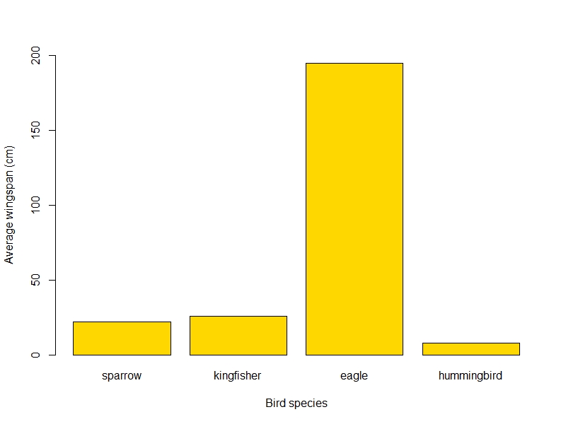
Here are (fictional) values of the wingspan (in cm) measured on four different species of birds. Can you produce a bar plot of the mean wingspan for each species and save it to your computer? (What could the function for calculating the mean be? Think simple)
| bird_sp | wingspan |
|---|---|
| sparrow | 22 |
| kingfisher | 26 |
| eagle | 195 |
| hummingbird | 8 |
| sparrow | 24 |
| kingfisher | 23 |
| eagle | 201 |
| hummingbird | 9 |
| sparrow | 21 |
| kingfisher | 25 |
| eagle | 185 |
| hummingbird | 9 |
Solution
Don’t peek until you’ve tried! Here we suggest a solution; note that yours could be different and also work! The object names and the look of your plot will probably be different and that’s totally ok - as long as the values themselves are correct.
Ready? Click this line to view the solution
# Calculate the mean wingspan for each bird species. The function to do that is simply: mean()
sparrow <- mean(22, 24, 21)
kingfisher <- mean(26, 23, 25)
eagle <- mean(195, 201, 185)
hummingbird <- mean(8, 9, 9)

# Chain them together in a vector
wingspan <- c(sparrow, kingfisher, eagle, hummingbird)

# Create a bird species vector (careful to match the order of the previous vector!)
bird_sp <- c("sparrow", "kingfisher", "eagle", "hummingbird")
# notice how we put quotation marks around the names. It's because we're creating (character) values; writing sparrow without the "" would call the object we created in the code above, which would return the value 22!

# Bird species is currently in character form, but it should be a factor. Let's fix that:
# (To be honest it does not make any difference to the output here, but it would for some other types of plot. Take good habits early!)
class(bird_sp)                      # currently character
bird_sp <- as.factor(bird_sp)       # transforming into factor
class(bird_sp)                      # now a factor!


# Then, combine the two vectors in a data frame
wings <- data.frame(bird_sp, wingspan)

# Plot the bar plot & save it to file

png("wingspan_plot.png", width=800, height=600)
barplot(wings$wingspan, names.arg = wings$bird_sp,    # notice how we call the bird_sp column instead of typing all the names
        xlab = "Bird species",
        ylab = "Average wingspan (cm)",               # adding axis titles
        ylim = c(0, 200),                             # setting the limits of the y axis to fit the eagle
        col = "gold"                                  # changing the colour because why not!
        )
dev.off()
And the final plot would look something like this:
Interested in taking your first steps in statistical modelling? Check out our in-depth tutorial ANOVA from A to (XY)Z!
Doing this tutorial as part of our Data Science for Ecologists and Environmental Scientists online course?
This tutorial is part of the Stats from Scratch stream from our online course. Go to the stream page to find out about the other tutorials part of this stream!
If you have already signed up for our course and you are ready to take the quiz, go to our quiz centre. Note that you need to sign up first before you can take the quiz. If you haven't heard about the course before and want to learn more about it, check out the course page.
Glossary:
To recap, here are a few important terms we learned in this lesson:
- argument: an element of a function, either essential or optional, that informs or alters how the function works. For instance, it can be a file path where the function should import from or save to:
file = \"file-path\". It can modify the colours in a plot:col = \"blue\". You can always find which arguments are taken by a function by typing?function-nameinto the command line. - class: the type of data contained in a variable: usually character (text/words), numeric (numbers), integer (whole numbers), or factor (grouping values, useful when you have multiple observations for sites or treatments in your data).
- command: a chunk of code that performs an action, typically contains one or more functions. You run a command by pressing "Run" or using a keyboard shortcut like
Cmd+Enter,Ctrl+EnterorCtrl+R - comment: a bit of text in a script that starts with a hashtag
#and isn’t read as a command. Comments make your code readable to other people: use them to create sections in your script and to annotate each step of your analysis - console: the window where you can type code directly in the command line (
2+2followed byEnterwill return4), and where the outputs of commands you run will show. - data frame: a type of R object which consists of many rows and columns; think Excel spreadsheet. Usually the columns are different variables (e.g. age, colour, weight, wingspan), and rows are observations of these variables (e.g. for bird1, bird2, bird3) .
- csv file: a type of file commonly used to import data in R, where the values of different variables are compressed together (a string, or line of values per row) and separated only by commas (indicating columns). R can also accept Excel (.xlsx) files, but we do not recommend it as formatting errors are harder to avoid.
- function: code that performs an action, and really how you do anything in R. Usually takes an input, does something to it, and returns an output (an object, a test result, a file, a plot). There are functions for importing, converting, and manipulating data, for performing specific calculations (can you guess what
min(10,15,5)andmax(10,15,5)would return?), making graphs, and more. - object: the building blocks of R. If R was a spoken language, functions would be verbs (actions) and objects would be nouns (the subjects or, well, objects of these actions!). Objects are called by typing their name without quotation marks. Objects store data, and can take different forms. The most common objects are data frames and vectors, but there are many more, such as lists and matrices.
- package: a bundle of functions that provide functionality to R. Many packages come automatically with R, others you can download for specific needs.
- script: Similar to a text editor, this is where you write and save your code for future reference. It contains a mix of code and comments and is saved as a simple text file that you can easily share so that anyone can reproduce your work.
- vector: a type of R object with one dimension: it stores a line of values which can be character, numeric, etc.
- working directory: the folder on your computer linked to your current R session, where you import data from and save files to. You set it at the beginning of your session with the
setwd()function. - workspace: this is your virtual working environment, which contains all the functions of the packages you have loaded, the data you have imported, the objects you have created, and so on. It’s usually best to start a work session with a clear workspace.