Material for this tutorial was adapted from the SciTools tutorial (SciTools is the group that maintain the Iris software.) It was adapted and modified under the GNU public licence v3.0 for this Coding Club tutorial and we acknowledge appreciate the use of original source materials from SciTools - Thank you!_
Welcome to this tutorial in the Python series about the Iris python package. Iris is a powerful tool used for manipulating multi-dimensional earth science data. Iris is really useful when you are dealing with data from sources such as weather and climate models, particularly when it is stored in common formats such as NetCDF (a common data file format used in the climate science community.)
Iris has data manipulation and visualisation features such as:
- A visualisation interface based on matplotlib and cartopy
- Unit conversion
- Subsetting and extraction of data
- Merge and concatenate
- Aggregations and reductions (including min, max, mean and weighted averages)
- Interpolation and regridding (including nearest-neighbor, linear and area-weighted)
If you need any of the above features and you find that you are regularly writing your own custom functions in Python to do these things, you may find that Iris already has these features availabe, and it can save you a lot of time in your work.
Tutorial aims:
- Understand what Iris is
- Learn about the core Iris data structure: the Iris cube
- Learn how to load data selectively from large datasets
- Learn how to manipulate and plot data with iris
1. What is Iris?
{: #understanding}}
Iris was developed originally by the Met Office (UK) out of a need for dealing with the many file formats used in the weather, climate, and ocean sciences scientific community. Many users of Iris had previously had to write their own code from scratch to handle and manipulate these file-formats, such as NetCDF, GRIB, and other common (and not-so-common) formats, alternatively they had to use one of the many separately available packages for each type of file format. (Such as python-netcdf4 for python, etc.). This resulted in a lot of duplicated effort from researchers re-writing what was effectively the same or very similar code. In addition, many operations on weather and climate data are essentially very similar, such as converting between different units, extracting subsets of the data, merging datasets, interpolating data, and so on. Iris was developed to bring together these operations and provide a file-format agnostic package to deal with these commonly used operations.
Iris operates around a central data structure used to store multi-dimiensional data when you are working on it called a cube. This typically represents gridded data that has many levels as well as x and y dimensions (Though Iris is still useful for 2 dimesnional data as well.)
The third dimension in an Iris could be model levels, different heights in the atmosphere, or depths in the ocean. It could also be used to represent different time-slices in a model run. In short, the Iris cube data structure is very flexible and can be used to represent a large variety of different datasets.
We are going to have a look at how the Iris cube data structure works now, but first, let’s test that we have iris installed:
import iris
import numpy as np

print(iris.__version__)
print(np.__version__)
This should print out the version numbers of iris and numpy, the two main requirements for this tutorial.
If you do not have these two packages installed, see this guide on installigin iris. (We assume you already have Python installed in your computing environmnet.
2. The Iris Cube
Learning outcome: by the end of this section, you will be able to explain the capabilities and functionality of Iris cubes and coordinates.
The top level object in Iris is called a cube. A cube contains data and metadata about a single phenomenon and is an implementation of the data model interpreted from the Climate and Forecast (CF) Metadata Conventions.
Each cube has:
- A data array (typically a NumPy array).
- A “name”, preferably a CF “standard name” to describe the phenomenon that the cube represents.
- A collection of coordinates to describe each of the dimensions of the data array. These coordinates are split into two types:
- Dimensioned coordinates are numeric, monotonic and represent a single dimension of the data array. There may be only one dimensioned coordinate per data dimension.
- Auxilliary coordinates can be of any type, including discrete values such as strings, and may represent more than one data dimension.
A fuller explanation is available in the Iris User Guide.
Let’s take a simple example to demonstrate the cube concept.
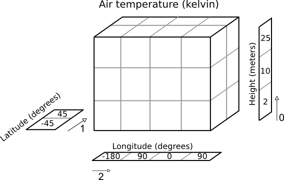
Suppose we have a (3, 2, 4) NumPy array:
Where dimensions 0, 1, and 2 have lengths 3, 2 and 4 respectively.
The Iris cube to represent this data may consist of:
- a standard name of “air_temperature” and units of “kelvin”
- a data array of shape
(3, 2, 4) - a coordinate, mapping to dimension 0, consisting of:
- a standard name of “height” and units of “meters”
- an array of length 3 representing the 3 height points
- a coordinate, mapping to dimension 1, consisting of:
- a standard name of “latitude” and units of “degrees”
- an array of length 2 representing the 2 latitude points
- a coordinate system such that the latitude points could be fully located on the globe
- a coordinate, mapping to dimension 2, consisting of:
- a standard name of “longitude” and units of “degrees”
- an array of length 4 representing the 4 longitude points
- a coordinate system such that the longitude points could be fully located on the globe
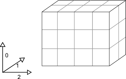
Pictorially the cube has taken on more information than a simple array:
Working with a cube
Whilst it is possible to construct a cube by hand, a far more common approach to getting hold of a cube is to use the Iris load function to access data that already exists in a file.
fname = iris.sample_data_path('uk_hires.pp')
cubes = iris.load(fname)
print(cubes)
We can see that we’ve loaded two cubes, one representing the “surface_altitude” and the other representing “air_potential_temperature”. We can infer even more detail from this printout; for example, what are the dimensions and shape of the “air_potential_temperature” cube?
Above we’ve printed the iris.cube.CubeList instance representing all of the cubes found in the given filename. However, we can see more detail by printing individual cubes:
fname = iris.sample_data_path('uk_hires.pp')
cubes = iris.load(fname)

air_pot_temp = cubes[0]
print(air_pot_temp)
Cube attributes
We can create a single cube from the load_cube command. Iris also provides some sample data that we can work with in the iris.sample_data_path function. Printing a cube object in Python will give you an overview of the data it contains and the layout of that data:
cube = iris.load_cube(iris.sample_data_path('A1B_north_america.nc'))
print(cube)
Which should print:
air_temperature / (K)               (time: 240; latitude: 37; longitude: 49)
     Dimension coordinates:
          time                           x              -              -
          latitude                       -              x              -
          longitude                      -              -              x
     Auxiliary coordinates:
          forecast_period                x              -              -
     Scalar coordinates:
          forecast_reference_time: 1859-09-01 06:00:00
          height: 1.5 m
     Attributes:
          Conventions: CF-1.5
          Model scenario: A1B
          STASH: m01s03i236
          source: Data from Met Office Unified Model 6.05
     Cell methods:
          mean: time (6 hour)
To access a cube’s data array the data property exists. This is either a NumPy array or in some cases a NumPy masked array. It is very important to note that for most of the supported filetypes in Iris, the cube’s data isn’t actually loaded until you request it via this property (either directly or indirectly). After youve accessed the data once, it is stored on the cube and thus wont be loaded from disk again.
To find the shape of a cube’s data it is possible to call cube.data.shape or cube.data.ndim, but this will trigger any unloaded data to be loaded. Therefore shape and ndim are properties available directly on the cube that do not unnecessarily load data.
cube = iris.load_cube(iris.sample_data_path('A1B_north_america.nc'))
print(cube.shape)
print(cube.ndim)
print(type(cube.data))
Which should display:
(240, 37, 49)
3
<class 'numpy.ma.core.MaskedArray'>
The standard_name, long_name and to an extent var_name are all attributes to describe the phenomenon that the cube represents. The name() method is a convenience that looks at the name attributes in the order they are listed above, returning the first non-empty string. To rename a cube, it is possible to set the attributes manually, but it is generally easier to use the rename() method.
From now on, we are not going to re-type the cube = iris.load_cube(...) line, it is assumed you will just change or append the lines below to your existing Python code. This is done to avoid having to reload the data into memory in each example!
print(cube.standard_name)
print(cube.long_name)
print(cube.var_name)
print(cube.name())
Check that you get the output:
air_temperature
None
air_temperature
air_temperature
There are a set of conventions used in climate data files called the “CF-conventions”. These are standard names and units that are used to make interchanging and sharing data more consistent and straightforward. More about the CF-conventions can be read here: XXXX
Iris can deal with CF-convention formatted data, but it also supports non-CF named data too. To illustrate this, we can change the name of our cube (in other words, rename our dataset) and see how Iris deals with this:
cube.rename("A name that isn't a valid CF standard name")
print(cube.standard_name)
print(cube.long_name)
print(cube.var_name)
print(cube.name())
Should print:
None
A name that isn't a valid CF standard name
None
A name that isn't a valid CF standard name
The units attribute on a cube tells us the units of the numbers held in the data array. We can manually change the units, or better, we can convert the cube to another unit using the convert_units method, which will automatically update the data array.
print(cube.units)
print(cube.data.max())
cube.convert_units('Celsius')
print(cube.units)
print(cube.data.max())
Should give you:
K
306.0733
Celsius
32.9233
A cube has a dictionary for extra general purpose attributes, which can be accessed with the cube.attributes attribute:
print(cube.attributes)
print(cube.attributes['STASH'])
Prints:
{'Conventions': 'CF-1.5', 'STASH': STASH(model=1, section=3, item=236), 'Model scenario': 'A1B', 'source': 'Data from Met Office Unified Model 6.05'}
m01s03i236
Coordinates
As we’ve seen, cubes need coordinate information to help us describe the underlying phenomenon. Typically a cube’s coordinates are accessed with the coords or coord methods. The latter must return exactly one coordinate for the given parameter filters, where the former returns a list of matching coordinates, possibly of length 0.
For example, to access the time coordinate, and print the first 4 times:
time = cube.coord('time')
print(time[:4])
Will display a representation of the time coordinate, as well as the metadata associated with it. This will be formatted according to the time units specified, if there are any present:
DimCoord([1860-06-01 00:00:00, 1861-06-01 00:00:00, 1862-06-01 00:00:00,
       1863-06-01 00:00:00], bounds=[[1859-12-01 00:00:00, 1860-12-01 00:00:00],
       [1860-12-01 00:00:00, 1861-12-01 00:00:00],
       [1861-12-01 00:00:00, 1862-12-01 00:00:00],
       [1862-12-01 00:00:00, 1863-12-01 00:00:00]], standard_name='time', calendar='360_day', var_name='time')
The coordinate interface is very similar to that of a cube. The attributes that exist on both cubes and coordinates are: standard_name, long_name, var_name, units,attributes and shape. Similarly, the name(), rename() and convert_units() methods also exist on a coordinate.
A coordinate does not have data, instead it has points and bounds (bounds may be None). In Iris, time coordinates are currently represented as “a number since an epoch”. So for example:
print(repr(time.units))
print(time.points[:4])
print(time.bounds[:4])
Will show the time values as whole numbers, rather than formatting them as a more human readable time-date value:
Unit('hours since 1970-01-01 00:00:00', calendar='360_day')
[-946800. -938160. -929520. -920880.]
[[-951120. -942480.]
 [-942480. -933840.]
 [-933840. -925200.]
 [-925200. -916560.]]
These numbers can be converted to datetime objects with the unit’s num2date method. Dates can be converted back again with the date2num method:
import datetime

print(time.units.num2date(time.points[:4]))
print(time.units.date2num(datetime.datetime(1970, 2, 1)))
Giving:
[cftime.Datetime360Day(1860, 6, 1, 0, 0, 0, 0, 4, 151)
 cftime.Datetime360Day(1861, 6, 1, 0, 0, 0, 0, 0, 151)
 cftime.Datetime360Day(1862, 6, 1, 0, 0, 0, 0, 3, 151)
 cftime.Datetime360Day(1863, 6, 1, 0, 0, 0, 0, 6, 151)]
720.0
Another important attribute on a coordinate is its coordinate system. Coordinate systems may be None for trivial coordinates, but particularly for spatial coordinates, they may be complex definitions of things such as the projection, ellipse and/or datum.
We can retrieve information about our coordinate system for example, by examining the latitude variable. The coordinate system is an attribute that can be printed, like so:
lat = cube.coord('latitude')
print(lat.coord_system)
Showing:
GeogCS(6371229.0)
3. Loading and saving data
Learning outcome: by the end of this section, you will be able to use Iris to load datasets from disk as Iris cubes and save Iris cubes back to disk.
Loading and savingdata is one aspect where Iris really shines over standard numpy or pandas methods of loading climate data. Notice that in the above examples we didn’t have to specify anything about the file formats of the netCDF files that we used.
Iris load functions
There are three main load functions in Iris: load, load_cube and load_cubes.
- load is a general purpose loading function. Typically this is where all data analysis will start, before more loading is refined with the more controlled loading from the other two functions.
- load_cube returns a single cube from the given source(s) and constraint. There will be exactly one cube, or an exception will be raised.
- load_cubes returns a list of cubes from the given sources(s) and constraint(s). There will be exactly one cube per constraint, or an exception will be raised.
Note: load_cube is a special case of load, which can be seen with:
fname = iris.sample_data_path('air_temp.pp')
c1, = iris.load(fname)
c2 = iris.load_cube(fname)
c1 == c2    # True
In other words, iris.load() has figured out that our sample dataset contains a single variable, and so returns a single cube, just like load_cube would do as well.
Saving cubes
The iris.save function provides a convenient interface to save Cube and CubeList instances.
To save some cubes to a NetCDF file:
fname = iris.sample_data_path('uk_hires.pp')
cubes = iris.load(fname)
iris.save(cubes, 'saved_cubes.nc')
We are just loading the netcdf file, converting it to the general purpose Iris cube data structure, and then saving it back to dsik. Iris takes care of converting the format, and the format is automatically taken care of.
You can skip this section if you are less familiar with the command line netCDF tools
To inspect our new netcdf file, we can check it with ncdump - the utility installed for inspecting netcdf files. (This should already be installed if you are on one of the Edinburgh linux servers. Type the following at the linux command line:
ncdump -h saved_cubes.nc | head -n 20
Which should output something like:
netcdf saved_cubes {
dimensions:
	time = 3 ;
	model_level_number = 7 ;
	grid_latitude = 204 ;
	grid_longitude = 187 ;
	bnds = 2 ;
variables:
	float air_potential_temperature(time, model_level_number, grid_latitude, grid_longitude) ;
		air_potential_temperature:standard_name = "air_potential_temperature" ;
		air_potential_temperature:units = "K" ;
		air_potential_temperature:um_stash_source = "m01s00i004" ;
		air_potential_temperature:grid_mapping = "rotated_latitude_longitude" ;
		air_potential_temperature:coordinates = "forecast_period forecast_reference_time level_height sigma surface_altitude" ;
	int rotated_latitude_longitude ;
		rotated_latitude_longitude:grid_mapping_name = "rotated_latitude_longitude" ;
		rotated_latitude_longitude:longitude_of_prime_meridian = 0. ;
		rotated_latitude_longitude:earth_radius = 6371229. ;
		rotated_latitude_longitude:grid_north_pole_latitude = 37.5 ;
		rotated_latitude_longitude:grid_north_pole_longitude = 177.5 ;
}
Out-of-core Processing
Out-of-core processing is a technical term that describes being able to process datasets that are too large to fit in memory at once. In Iris, this functionality is referred to as lazy data. It means that you can use Iris to load, process and save datasets that are too large to fit in memory without running out of memory. This is achieved by loading only the dataset’s metadata and not the data array, unless this is specifically requested.
To determine whether your cube has lazy data:
fname = iris.sample_data_path('air_temp.pp')
cube = iris.load_cube(fname)
print(cube.has_lazy_data())
Iris tries to maintain lazy data as much as possible. We refer to the operation of loading a cube’s lazy data as ‘realising’ the cube’s data. A cube’s lazy data will only be loaded in a limited number of cases, including:
- When the user directly requests the cube’s data using
cube.data, - When there is no lazy data processing algorithm available to perform the requested data processing, such as for peak finding, and
- Where actual data values are necessary, such as for cube plotting.
Cube control and subsetting
Learning outcome: by the end of this section, you will be able to apply Iris functionality to take a useful subset of an Iris cube and to combine multiple Iris cubes into a new larger cube.
Constraints and Extract
We’ve already seen the basic load function, but we can also control which cubes are actually loaded with constraints. The simplest constraint is just a string, which filters cubes based on their name:
fname = iris.sample_data_path('uk_hires.pp')
print(iris.load(fname, 'air_potential_temperature'))
0: air_potential_temperature / (K) (time: 3; model_level_number: 7; grid_latitude: 204; grid_longitude: 187)
Iris’s constraints mechanism provides a powerful way to filter a subset of data from a larger collection. We’ve already seen that constraints can be used at load time to return data of interest from a file, but we can also apply constraints to a single cube, or a list of cubes, using their respective extract methods:
cubes = iris.load(fname)
print(cubes.extract('air_potential_temperature'))
Which will give us the same output as the previous output:
0: air_potential_temperature / (K) (time: 3; model_level_number: 7; grid_latitude: 204; grid_longitude: 187)
The simplest constraint, namely a string that matches a cube’s name, is conveniently converted into an actual iris.Constraint instance wherever needed. However, we could construct this constraint manually and compare with the previous result:
pot_temperature_constraint = iris.Constraint('air_potential_temperature')
print(cubes.extract(pot_temperature_constraint))
0: air_potential_temperature / (K) (time: 3; model_level_number: 7; grid_latitude: 204; grid_longitude: 187)
The Constraint constructor also takes arbitrary keywords to constrain coordinate values. For example, to extract model level number 10 from the air potential temperature cube:
pot_temperature_constraint = iris.Constraint('air_potential_temperature',
                                             model_level_number=10)
print(cubes.extract(pot_temperature_constraint))
0: air_potential_temperature / (K) (time: 3; grid_latitude: 204; grid_longitude: 187)
We can pass a list of possible values, and even combine two constraints with &:
print(cubes.extract('air_potential_temperature' &
                    iris.Constraint(model_level_number=[4, 10])))
0: air_potential_temperature / (K) (time: 3; model_level_number: 2; grid_latitude: 204; grid_longitude: 187)
We can define arbitrary functions that operate on each cell of a coordinate. This is a common thing to do for floating point coordinates, where exact equality is non-trivial.
def less_than_10(cell):
    """Return True for values that are less than 10."""
    return cell < 10

print(cubes.extract(iris.Constraint('air_potential_temperature',
                                    model_level_number=less_than_10)))
0: air_potential_temperature / (K) (time: 3; model_level_number: 3; grid_latitude: 204; grid_longitude: 187)
Time Constraints
It is common to want to build a constraint for time. This can be achieved by comparing cells containing datetimes.There are a few different approaches for producing time constraints in Iris. We will focus here on one approach for constraining on time in Iris.
This approach allows us to access individual components of cell datetime objects and run comparisons on those:
time_constraint = iris.Constraint(time=lambda cell: cell.point.hour == 11)
print(air_pot_temp.extract(time_constraint).summary(True))
air_potential_temperature / (K) (model_level_number: 7; grid_latitude: 204; grid_longitude: 187)
Indexing
Cubes can be indexed in a familiar manner to that of NumPy arrays:
fname = iris.sample_data_path('uk_hires.pp')
cube = iris.load_cube(fname, 'air_potential_temperature')
print(cube.summary(shorten=True))
air_potential_temperature / (K) (time: 3; model_level_number: 7; grid_latitude: 204; grid_longitude: 187)
We can define a constraint on our cube by creating a list of indices to be used, similarly to NumPy:
subcube = cube[..., ::2, 15:35, :10]
subcube.summary(shorten=True)
'air_potential_temperature / (K) (time: 3; model_level_number: 4; grid_latitude: 20; grid_longitude: 10)'
Note: the result of indexing a cube is always a copy and never a view on the original data.
Iteration
We can loop through all desired subcubes in a larger cube using the cube methods slices and slices_over.
fname = iris.sample_data_path('uk_hires.pp')
cube = iris.load_cube(fname,
                      iris.Constraint('air_potential_temperature',
                                      model_level_number=1))
print(cube.summary(True))
air_potential_temperature / (K) (time: 3; grid_latitude: 204; grid_longitude: 187)
The slices method returns all the slices of a cube on the dimensions specified by the coordinates passed to the slices method.
So in this example, each grid_latitude / grid_longitude slice of the cube is returned:
for subcube in cube.slices(['grid_latitude', 'grid_longitude']):
    print(subcube.summary(shorten=True))
air_potential_temperature / (K)     (grid_latitude: 204; grid_longitude: 187)
air_potential_temperature / (K)     (grid_latitude: 204; grid_longitude: 187)
air_potential_temperature / (K)     (grid_latitude: 204; grid_longitude: 187)
We can use slices_over to return one subcube for each coordinate value in a specified coordinate. This helps us when trying to retrieve all the slices along a given cube dimension.
For example, let’s consider retrieving all the slices over the time dimension (i.e. each time step in its own cube with a scalar time coordinate) using slices. As per the above example, to achieve this using slices we would have to specify all the cube’s dimensions except the time dimension.
Let’s take a look at slices_over providing this functionality:
fname = iris.sample_data_path('uk_hires.pp')
cube = iris.load_cube(fname, 'air_potential_temperature')
for subcube in cube.slices_over('model_level_number'):
    print(subcube.summary(shorten=True))
air_potential_temperature / (K)     (time: 3; grid_latitude: 204; grid_longitude: 187)
air_potential_temperature / (K)     (time: 3; grid_latitude: 204; grid_longitude: 187)
air_potential_temperature / (K)     (time: 3; grid_latitude: 204; grid_longitude: 187)
air_potential_temperature / (K)     (time: 3; grid_latitude: 204; grid_longitude: 187)
air_potential_temperature / (K)     (time: 3; grid_latitude: 204; grid_longitude: 187)
air_potential_temperature / (K)     (time: 3; grid_latitude: 204; grid_longitude: 187)
air_potential_temperature / (K)     (time: 3; grid_latitude: 204; grid_longitude: 187)
Discussion: Indexing and slicing
- What are the similarities between indexing and slicing?
- What are the differences?
- Which cube slicing method would be easiest to use to return all subcubes along the realization dimension?
- Which cube slicing method would be easiest to use to return all horizontal 2D slices in a 4D cube?
- In what situations would indexing be the best way to subset a cube? What about slicing?
4. Data Processing and Visualisation
Learning outcome: by the end of this section, you will be able to use Iris to analyse and visualise weather and climate datasets.
Plotting
Iris comes with two plotting modules called iris.plot and iris.quickplot that wrap some of the common matplotlib plotting functions such that cubes can be passed as input rather than the usual NumPy arrays. The two modules are very similar, with the primary difference being that quickplot will add extra information to the axes, such as:
- a colorbar,
- labels for the x and y axes, and
- a title where possible.
import iris.plot as iplt
import iris.quickplot as qplt
import matplotlib.pyplot as plt

cube = iris.load_cube(iris.sample_data_path('A1B_north_america.nc'))
ts = cube[-1, 20, ...]
print(ts)
Will print out the following summary of the sliced cube:
air_temperature / (K)               (longitude: 49)
     Dimension coordinates:
          longitude                           x
     Scalar coordinates:
          forecast_period: 2075754 hours
          forecast_reference_time: 1859-09-01 06:00:00
          height: 1.5 m
          latitude: 40.0 degrees
          time: 2099-06-01 00:00:00, bound=(2098-12-01 00:00:00, 2099-12-01 00:00:00)
     Attributes:
          Conventions: CF-1.5
          Model scenario: A1B
          STASH: m01s03i236
          source: Data from Met Office Unified Model 6.05
     Cell methods:
          mean: time (6 hour)
Now we can do some plotting! Adding to the above script, we can write:
iplt.plot(ts)
plt.show()
For comparison, lets plot the result of iplt.plot next to qplt.plot:
plt.subplot(2, 1, 1)
iplt.plot(ts)

plt.subplot(2, 1, 2)
qplt.plot(ts)

plt.subplots_adjust(hspace=0.5)
plt.show()
Notice how the result of qplt has axis labels and a title; everything else about the axes is identical.
The plotting functions in Iris have strict rules on the dimensionality of the inputted cubes. For example, a 2d cube is needed in order to create a contour plot:
qplt.contourf(cube[:, 0, :])
plt.show()
Maps with cartopy
When the result of a plot operation is a map, Iris will automatically create an appropriate cartopy axes if one doesn’t already exist.
We can use matplotlib’s gca() function to get hold of the automatically created cartopy axes:
import cartopy.crs as ccrs

plt.figure(figsize=(12, 8))

plt.subplot(1, 2, 1)
qplt.contourf(cube[0, ...], 25)
ax = plt.gca()
ax.coastlines()

ax = plt.subplot(1, 2, 2, projection=ccrs.RotatedPole(100, 37))
qplt.contourf(cube[0, ...], 25)
ax.coastlines()

plt.show()
Cube maths
Basic mathematical operators exist on the cube to allow one to add, subtract, divide, multiply and perform other mathematical operations on cubes of a similar shape to one another:
a1b = iris.load_cube(iris.sample_data_path('A1B_north_america.nc'))
e1 = iris.load_cube(iris.sample_data_path('E1_north_america.nc'))

print(e1.summary(True))
print(a1b)
Should show us the summary:
air_temperature / (K)               (time: 240; latitude: 37; longitude: 49)
air_temperature / (K)               (time: 240; latitude: 37; longitude: 49)
     Dimension coordinates:
          time                           x              -              -
          latitude                       -              x              -
          longitude                      -              -              x
     Auxiliary coordinates:
          forecast_period                x              -              -
     Scalar coordinates:
          forecast_reference_time: 1859-09-01 06:00:00
          height: 1.5 m
     Attributes:
          Conventions: CF-1.5
          Model scenario: A1B
          STASH: m01s03i236
          source: Data from Met Office Unified Model 6.05
     Cell methods:
          mean: time (6 hour)
To find the difference between these two cubes we have created, we can do this by adding the following lines of code:
scenario_difference = a1b - e1
print(scenario_difference)
Giving us:
unknown / (K)                       (time: 240; latitude: 37; longitude: 49)
     Dimension coordinates:
          time                           x              -              -
          latitude                       -              x              -
          longitude                      -              -              x
     Auxiliary coordinates:
          forecast_period                x              -              -
     Scalar coordinates:
          forecast_reference_time: 1859-09-01 06:00:00
          height: 1.5 m
Notice that the resultant cube’s name is now unknown and that resultant cube’s attributes and cell_methods have disappeared; this is because these all differed between the two input cubes.
It is also possible to operate on cubes with numeric scalars, NumPy arrays and even cube coordinates:
print(e1 * e1.coord('latitude'))
unknown / (0.0174532925199433 K.rad) (time: 240; latitude: 37; longitude: 49)
     Dimension coordinates:
          time                            x              -              -
          latitude                        -              x              -
          longitude                       -              -              x
     Auxiliary coordinates:
          forecast_period                 x              -              -
     Scalar coordinates:
          forecast_reference_time: 1859-09-01 06:00:00
          height: 1.5 m
Cube broadcasting is also taking place, meaning that the two inputs (cube, coordinate, array, or even constant value) don’t need to have the same shape:
print(e1 + 5.0)
unknown / (K)                       (time: 240; latitude: 37; longitude: 49)
     Dimension coordinates:
          time                           x              -              -
          latitude                       -              x              -
          longitude                      -              -              x
     Auxiliary coordinates:
          forecast_period                x              -              -
     Scalar coordinates:
          forecast_reference_time: 1859-09-01 06:00:00
          height: 1.5 m
As we’ve just seen, we have the ability to update the cube’s data directly. Whenever we do this though, we should be mindful of updating appropriate metadata on the cube:
e1_hot = e1.copy()

e1_hot.data = np.ma.masked_less_equal(e1_hot.data, 280)
e1_hot.rename('air temperatures greater than 280K')
print(e1_hot)
air temperatures greater than 280K / (K) (time: 240; latitude: 37; longitude: 49)
     Dimension coordinates:
          time                                x              -              -
          latitude                            -              x              -
          longitude                           -              -              x
     Auxiliary coordinates:
          forecast_period                     x              -              -
     Scalar coordinates:
          forecast_reference_time: 1859-09-01 06:00:00
          height: 1.5 m
     Attributes:
          Conventions: CF-1.5
          Model scenario: E1
          STASH: m01s03i236
          source: Data from Met Office Unified Model 6.05
     Cell methods:
          mean: time (6 hour)
Cube aggregation and statistics
Many standard univariate aggregations exist in Iris. Aggregations allow one or more dimensions of a cube to be statistically collapsed for the purposes of statistical analysis of the cube’s data. Iris uses the term “aggregators” to refer to the statistical operations that can be used for aggregation.
A list of aggregators is available at [http://scitools.org.uk/iris/docs/latest/iris/iris/analysis.html].
fname = iris.sample_data_path('uk_hires.pp')
cube = iris.load_cube(fname, 'air_potential_temperature')
print(cube.summary(True))
air_potential_temperature / (K) (time: 3; model_level_number: 7; grid_latitude: 204; grid_longitude: 187)
To take the vertical mean of this cube:
print(cube.collapsed('model_level_number', iris.analysis.MEAN))
air_potential_temperature / (K)     (time: 3; grid_latitude: 204; grid_longitude: 187)
     Dimension coordinates:
          time                           x                 -                    -
          grid_latitude                  -                 x                    -
          grid_longitude                 -                 -                    x
     Auxiliary coordinates:
          forecast_period                x                 -                    -
          surface_altitude               -                 x                    x
     Derived coordinates:
          altitude                       -                 x                    x
     Scalar coordinates:
          forecast_reference_time: 2009-11-19 04:00:00
          level_height: 696.6666 m, bound=(0.0, 1393.3333) m
          model_level_number: 10, bound=(1, 19)
          sigma: 0.92292976, bound=(0.8458596, 1.0)
     Attributes:
          STASH: m01s00i004
          source: Data from Met Office Unified Model
          um_version: 7.3
     Cell methods:
          mean: model_level_number
Summary
In this tutorial we have looked at how to use the Python package iris: an extension of the Python language for loading common types of Earth and climate science data foramts, such as NetCDF. Iris also is a powerful software package for manipulating, analysing. and plotting the data once loaded, making it an integrated tool for Earth and climate data scientists.
Tutorial outcomes:
- You understand why Iris is a useful tool in the Python community for dealing with climate data.
- You know how to use the basic load functions for Iris
- You can create an Iris “cube” and understand the basics of the data structure
- You can apply more complex constraints to loading data from cubes, such as time and variable constraints.
- You understand the basics of cube slicing.
- You can create simple plots using the iris plotting interface. (Which is an extension of the
matplotliblibrary.)