Tutorial Aims:
- Understand what RMarkdown is and why you should use it
- Learn how to construct an RMarkdown file
- Export an RMarkdown file into many file formats
Steps:
- What is RMarkdown
- Download RMarkdown
- Create an RMarkdown (
.Rmd) file - YAML header material
- Markdown syntax
- Insert code from an R script into a
.Rmdfile - Create a
.pdffile from your.Rmdfile RNotebooks (the future of reproducible code? Maybe?)
1. What is R Markdown?
R Markdown allows you to create documents that serve as a neat record of your analysis. In the world of reproducible research, we want other researchers to easily understand what we did in our analysis, otherwise nobody can be certain that you analysed your data properly. You might choose to create an RMarkdown document as an appendix to a paper or project assignment that you are doing, upload it to an online repository such as Github, or simply to keep as a personal record so you can quickly look back at your code and see what you did. RMarkdown presents your code alongside its output (graphs, tables, etc.) with conventional text to explain it, a bit like a notebook.
RMarkdown makes use of Markdown syntax. Markdown is a very simple ‘markup’ language which provides methods for creating documents with headers, images, links etc. from plain text files, while keeping the original plain text file easy to read. You can convert Markdown documents to many other file types like .html or .pdf to display the headers, images etc..
When you create an RMarkdown file (.Rmd), you use conventional Markdown syntax alongside chunks of code written in R (or other programming languages!). When you knit the RMarkdown file, the Markdown formatting and the R code are evaluated, and an output file (HTML, PDF, etc) is produced.
To see what RMarkdown is capable of, have a look at this undergraduate dissertation, which gives a concise log of their statistical analysis, or the completed demo RMarkdown file for this tutorial.
All the resources for this tutorial, including some helpful cheatsheets can be downloaded from this repository. Download by clicking on Code -> Download ZIP, then unzipping the archive in a folder you will use for this tutorial.
Read through this tutorial and use the information you learn along the way to convert the tutorial R script (RMarkdown_Tutorial.R), which you can find in the repo, into a well commented, logically structured R Markdown (.Rmd) document. Afterwards, there are some challenge scripts that you can convert to .Rmd documents. If you want, you could also try converting one of your own R scripts.
Haven’t used R or RStudio before? No worries! Check out our Intro to R and RStudio tutorial, then come back here to master RMarkdown!
2. Download R Markdown
To get RMarkdown working in RStudio, the first thing you need is the rmarkdown package, which you can get from CRAN by running the following commands in R or RStudio:
install.packages("rmarkdown")
library(rmarkdown)
3. Create an RMarkdown file
To create a new RMarkdown file (.Rmd), select File -> New File -> R Markdown..._ in RStudio, then choose the file type you want to create. For now we will focus on a .html Document, which can be easily converted to other file types later.
The newly created .Rmd file comes with basic instructions, but we want to create our own RMarkdown script, so go ahead and delete everything in the example file.
Now save the .Rmd file to the repository you downloaded earlier from Github.
Now open the RMarkdown_Tutorial.R practice script from the repository you downloaded earlier in another tab in RStudio and use the instructions below to help you convert this script into a coherent RMarkdown document, bit by bit.
If you have any of your own R scripts that you would like to make into an R Markdown document, you can also use those!
4. The YAML Header
At the top of any RMarkdown script is a YAML header section enclosed by ---. By default this includes a title, author, date and the file type you want to output to. Many other options are available for different functions and formatting, see here for .html options and here for .pdf options. Rules in the header section will alter the whole document. Have a flick through quickly to familiarise yourself with the sorts of things you can alter by adding an option to the YAML header.
Insert something like this at the top of your new .Rmd script:
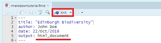
---
title: "Edinburgh Biodiversity"
author: John Doe
date: 22/Oct/2016
output: html_document
---
By default, the title, author, date and output format are printed at the top of your .html document. This is the minimum you should put in your header section.
Now that we have our first piece of content, we can test the .Rmd file by compiling it to .html. To compile your .Rmd file into a .html document, you should press the Knit button in the taskbar:
By default, RStudio opens a separate preview window to display the output of your .Rmd file. If you want the output to be displayed in the Viewer window in RStudio (the same window where you would see plotted figures / packages / file paths), select “View in Pane” from the drop down menu that appears when you click on the Knit button in the taskbar, or in the Settings gear icon drop down menu next to the Knit button.
A preview appears, and a .html file is also saved to the same folder where you saved your .Rmd file.
4. Markdown syntax
You can use regular markdown rules in your R Markdown document. Once you knit your document, the output will display text formatted according to the following simple rules.
Formatting Text
Here are a few common formatting commands:
*Italic*
Italic
**Bold**
Bold
This is `code` in text
This is code in text
# Header 1
Header 1
## Header 2
Header 2
Note that when a # symbol is placed inside a code chunk it acts as a normal R comment, but when placed in text it controls the header size.
* Unordered list item
1. Ordered list item
- Ordered list item
[Link](https://www.google.com)
$A = \pi \times r^{2}$

The $ symbols tells R markdown to use LaTeX equation syntax.
To practice this, try writing some formatted text in your .Rmd document and producing a .html page using the “Knit” button.
5. Code Chunks
Below the YAML header is the space where you will write your code, accompanying explanation and any outputs. Code that is included in your .Rmd document should be enclosed by three backwards apostrophes ``` (grave accents!). These are known as code chunks and look like this:
```{r}
norm <- rnorm(100, mean = 0, sd = 1)
```
You can quickly insert a code chunk in RStudio using a button in the toolbar:
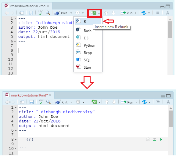
Inside the curly brackets is a space where you can assign rules for that code chunk. The code chunk above says that the code is R code. We’ll get onto some other curly brace rules later.
Have a go at grabbing some code from the example R script and inserting it into a code chunk in your .Rmd document.
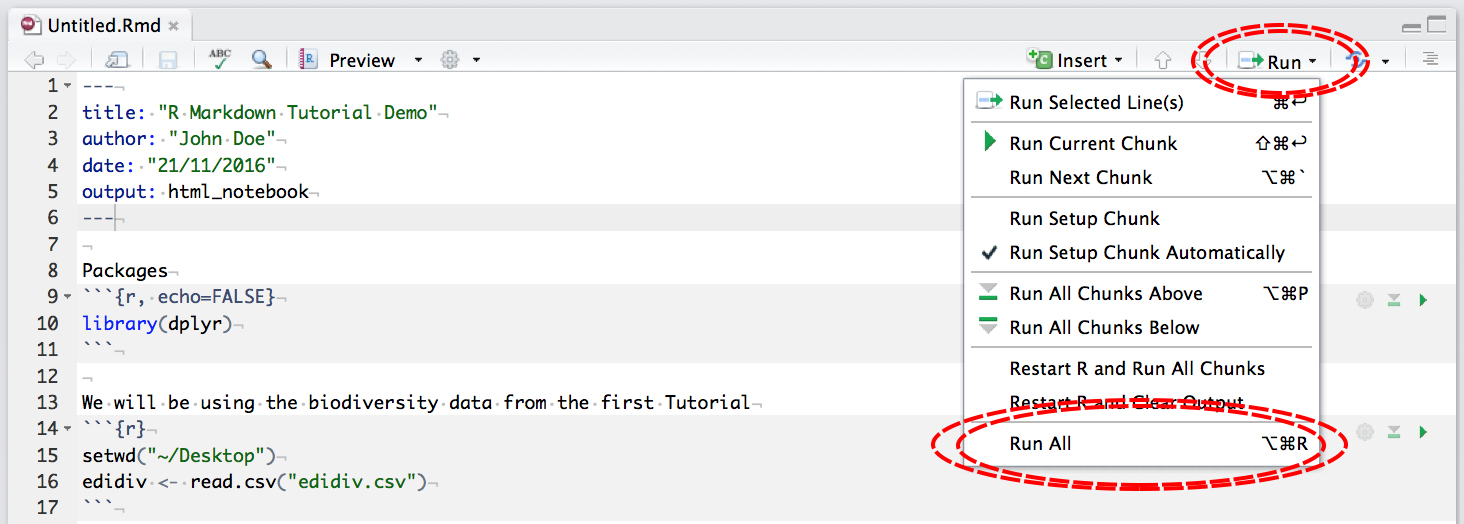
You can run an individual chunk of code at any time by clicking on the small green arrow:
![]()
The output of the code will appear just beneath the code chunk.
More on Code Chunks
It’s important to remember when you are creating an RMarkdown file that if you want to run code that refers to an object, for example:
```{r}
print(dataframe)
```
you must include instructions showing what dataframe is, just like in a normal R script. For example:
```{r}
A <- c("a", "a", "b", "b")
B <- c(5, 10, 15, 20)
dataframe <- data.frame(A, B)
print(dataframe)
```
Or if you are loading a dataframe from a .csv file, you must include the code in the .Rmd:
```{r}
dataframe <- read.csv("~/Desktop/Code/dataframe.csv")
```
Similarly, if you are using any packages in your analysis, you will have to load them in the .Rmd file using library() as in a normal R script.
```{r}
library(dplyr)
```
Hiding code chunks
If you don’t want the code of a particular code chunk to appear in the final document, but still want to show the output (e.g. a plot), then you can include echo = FALSE in the code chunk instructions.
```{r, echo = FALSE}
A <- c("a", "a", "b", "b")
B <- c(5, 10, 15, 20)
dataframe <- data.frame(A, B)
print(dataframe)
```
Similarly, you might want to create an object, but not include both the code and the output in the final .html file. To do this you can use, include = FALSE. Be aware though, when making reproducible research it’s often not a good idea to completely hide some part of your analysis:
```{r, include = FALSE}
richness <-
  edidiv %>%
    group_by(taxonGroup) %>%
    summarise(Species_richness = n_distinct(taxonName))
```
In some cases, when you load packages into RStudio, various warning messages such as “Warning: package ‘dplyr’ was built under R version 3.4.4” might appear. If you do not want these warning messages to appear, you can use warning = FALSE.
```{r, warning = FALSE}
library(dplyr)
```
REMEMBER: R Markdown doesn’t pay attention to anything you have loaded in other R scripts, you MUST load all objects and packages in the R Markdown script.
More Code Chunk Instructions
| Rule | Example (default) |
Function |
|---|---|---|
| eval | eval=TRUE | Is the code run and the results included in the output? |
| include | include=TRUE | Are the code and the results included in the output? |
| echo | echo=TRUE | Is the code displayed alongside the results? |
| warning | warning=TRUE | Are warning messages displayed? |
| error | error=FALSE | Are error messages displayed? |
| message | message=TRUE | Are messages displayed? |
| tidy | tidy=FALSE | Is the code reformatted to make it look “tidy”? |
| results | results="markup" | How are results treated? "hide" = no results "asis" = results without formatting "hold" = results only compiled at end of chunk (use if many commands act on one object) |
| cache | cache=FALSE | Are the results cached for future renders? |
| comment | comment="##" | What character are comments prefaced with? |
| fig.width, fig.height | fig.width=7 | What width/height (in inches) are the plots? |
| fig.align | fig.align="left" | "left" "right" "center" |
Inserting Figures
Inserting a graph into RMarkdown is easy, the more energy-demanding aspect might be adjusting the formatting.
By default, RMarkdown will place graphs by maximising their height, while keeping them within the margins of the page and maintaining aspect ratio. If you have a particularly tall figure, this can mean a really huge graph. In the following example we modify the dimensions of the figure we created above. To manually set the figure dimensions, you can insert an instruction into the curly braces:
```{r, fig.width = 4, fig.height = 3}
A <- c("a", "a", "b", "b")
B <- c(5, 10, 15, 20)
dataframe <- data.frame(A, B)
print(dataframe)
boxplot(B~A,data=dataframe)
```
Inserting Tables
Standard R Markdown
While R Markdown can print the contents of a data frame easily by enclosing the name of the data frame in a code chunk:
```{r}
dataframe
```
this can look a bit messy, especially with data frames with a lot of columns. Including a formal table requires more effort.
kable() function from knitr package
The most aesthetically pleasing and simple table formatting function I have found is kable() in the knitr package. The first argument tells kable to make a table out of the object dataframe and that numbers should have two significant figures. Remember to load the knitr package in your .Rmd file as well.
```{r}
library(knitr)
kable(dataframe, digits = 2)
```
pander function from pander package
If you want a bit more control over the content of your table you can use pander() in the pander package. Imagine I want the 3rd column to appear in italics:
```{r}
library(pander)
plant <- c("a", "b", "c")
temperature <- c(20, 20, 20)
growth <- c(0.65, 0.95, 0.15)
dataframe <- data.frame(plant, temperature, growth)
emphasize.italics.cols(3)   # Make the 3rd column italics
pander(dataframe)           # Create the table
```
Find more info on pander here.
Manually creating tables using markdown syntax
You can also manually create small tables using markdown syntax. This should be put outside of any code chunks.
For example:
| Plant | Temp. | Growth |
|:------|:-----:|-------:|
| A     | 20    | 0.65   |
| B     | 20    | 0.95   |
| C     | 20    | 0.15   |
will create something that looks like this:
| Plant | Temp. | Growth |
|---|---|---|
| A | 20 | 0.65 |
| B | 20 | 0.95 |
| C | 20 | 0.15 |
The :-----: tells markdown that the line above should be treated as a header and the lines below should be treated as the body of the table. Text alignment of the columns is set by the position of ::
| Syntax | Alignment |
|---|---|
| `:----:` | Centre |
| `:-----` | Left |
| `-----:` | Right |
| `------` | Auto |
Creating tables from model outputs
Using tidy() from the package broom, we are able to create tables of our model outputs, and insert these tables into our markdown file. The example below shows a simple example linear model, where the summary output table can be saved as a new R object and then added into the markdown file.
```{r warning=FALSE}
library(broom)
library(pander)
A <- c(20, 15, 10)
B <- c(1, 2, 3)

lm_test <- lm(A ~ B)            # Creating linear model

table_obj <- tidy(lm_test)      # Using tidy() to create a new R object called table

pander(table_obj, digits = 3)   # Using pander() to view the created table, with 3 sig figs
```
By using warning=FALSE as an argument, any warnings produced will be outputted in the console when knitting but will not appear in the produced document.
7. Creating .pdf files in Rmarkdown
Creating .pdf documents for printing in A4 requires a bit more fiddling around. RStudio uses another document compiling system called LaTeX to make .pdf documents.
The easiest way to use LaTeX is to install the TinyTex distribution from within RStudio. First, restart your R session (Session -> Restart R), then run these line in the console:
install.packages("tinytex")
tinytex::install_tinytex()
Becoming familiar with LaTeX will give you a lot more options to make your R Markdown .pdf look pretty, as LaTeX commands are mostly compatible with R Markdown, though some googling is often required.
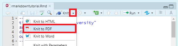
To compile a .pdf instead of a .html document, change output: from html_document to pdf_document, or use the dropdown menu from the “Knit” button:
Common problems when compiling a .pdf
- Text is running off the page
Add a global_options argument at the start of your .Rmd file:
```{r global_options, include = FALSE}
knitr::opts_chunk$set(message=FALSE,
tidy.opts=list(width.cutoff=60))
```
This code chunk won’t be displayed in the final document due to the include = FALSE call and should be placed immediately after the YAML header to affect everything below that.
tidy.opts = list(width.cutoff = 60) defines the margin cutoff point and wraps text to the next line. Play with the value to get it right.
- I lose my syntax highlighting
Use the xelatex engine to compile your .pdf:
---
author: John Doe
output:
  pdf_document:
    latex_engine: xelatex
---
By default, R markdown uses the base LaTeX engine to compile pdfs, but this may limit certain options when it comes to formatting. There are lots of other engines to play around with as well.
- My page margins are too big/small
Add a geometry argument to the YAML header
---
title: "R Markdown Tutorial Demo"
author: "John Godlee"
date: "30/11/2016"
output:
  pdf_document:
    latex_engine: xelatex
geometry: left = 0.5cm, right = 1cm, top = 1cm, bottom = 1cm
---
geometry is a LaTeX command.
- My plot/table/code is split over two pages
Add a page break before the dodgy element:
\pagebreak
```{r}
Codey codey code code
```
- I want to change the font
Add a font argument to your header section
---
title: "R Markdown Tutorial Demo"
author: "John Godlee"
date: "30/11/2016"
output:
  pdf_document:
    latex_engine: xelatex
mainfont: Arial
---
mainfont is a LaTeX command.
Have a go yourself
At this point, if you haven’t been following through already, have a go at converting the tutorial R script (RMarkdown_Tutorial.R) into a .Rmd document using the information above as a guide.
Remember that a good R markdown document should provide a reproducible log of your code, properly commented, with subtitles, comments and code relevant output so the reader knows what is going on.
8. R Notebooks
RMarkdown outputs to a non-interactive file format like .html or .pdf. When presenting your code, this means you have to make a choice, do you want interactive but messy looking code (.Rmd) or non-interactive but neat looking code (.html, .pdf)? R notebooks provide a file format that combines the interactivity of a .Rmd file with the attractiveness of .html output.
R notebooks output to the imaginatively named .nb.html format. .nb.html files can be loaded into a web browser to see the output, or loaded into a code editor like RStudio to see the code. You are able to interactively select which code chunks to hide or show code chunks.
Notebooks use the same syntax as .Rmd files so it is easy to copy and paste the script from a .Rmd into a Notebook. To create a new R Notebook file, select File -> New File -> R Notebook. Create a notebook from your newly created .Rmd file by copying and pasting the script. If you choose to copy and paste the script, make sure that under your YAML header, output: html_notebook instead of output: html_document.
Alternatively, to turn any existing .Rmd file into an R notebook, add html_notebook: default under the output: argument in the YAML header. If you have more than one output document type, the “Knit” button will only produce the first type. You can use the dropdown menu form the Knit button to produce one of the other types.
---
title: "R Markdown Tutorial Demo"
author: "John Godlee"
date: "30/11/2016"
output:
  html_notebook: default
  pdf_document:
    latex_engine: xelatex
mainfont: Arial
---
To output to .nb.html, first make sure all your code chunks have been run:
then click Preview:
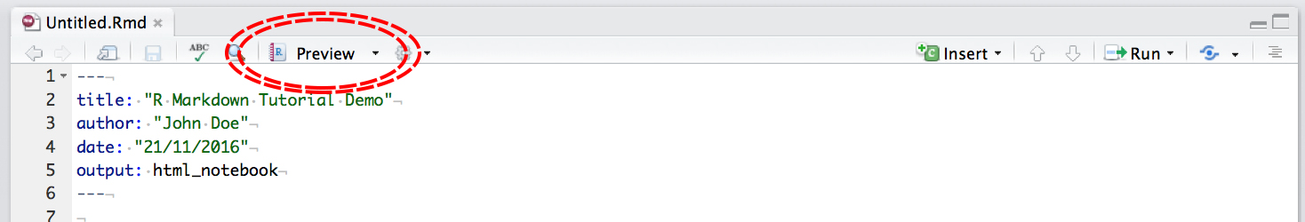
Notice that with R Notebooks you can still output to .html or .pdf, the same as a .Rmd file.
R notebooks have only been around for about a couple of years so they’re not perfect yet, but may replace R markdown in the future for many applications.
Difference between RMarkdown and RNotebooks
R Markdown documents are ‘knitted’, while R Notebooks are ‘previewed’.
Although the notebook preview looks similar to the knitted markdown document, the notebook preview does not execute any code chunks, but only shows you a rendered copy of the Markdown output of your document along with the most recent chunk output. The preview is also generated automatically whenever the notebook is saved. This would be especially useful if we have the preview showing in the Viewer window next to the console. This means that in R Notebooks, we are able to visually assess the output as we develop the document without having to knit the whole document again.
For example, with the following code chunk example (from the RMarkdown_Tutorial.R practice script), we are creating a table of species richness for each taxonomic group.
```{r}
richness <-
  edidiv %>%
  group_by(taxonGroup) %>%
  summarise(Species_richness = n_distinct(taxonName))
```
To bring up the table output, we can add richness, pander(richness), kable(richness) to the end of that code chunk. If we had initially forgotten to add in either one of those functions, the table would not have been produced in both the knitted markdown document and the notebook preview. Imagine that we are now editing the R Markdown document / R Notebook document to include this function to bring up the table in the outputted document.
For RMarkdown: we would type in pander(richness), run that specific code chunk, and then have to click the Knit button in the taskbar to knit the whole document again.
For R Notebooks, we type in pander(richness), run that specific code chunk, and save the document, and the preview in the Viewer window would be updated on its own - there is no need to click the Preview button in the taskbar and run the code for the whole document.
Note: R Markdown Notebooks are only available in RStudio 1.0 or higher.
Bonus task!
Either in a small group or on your own, convert one of the three demo R scripts into a well commented and easy to follow R Markdown document, or R Markdown Notebook. The files (RMarkdown_Demo_1.R, RMarkdown_Demo_2.R, RMarkdown_Demo_3.R) can be found in the repo you downloaded earlier.
Tutorial Outcomes:
- You are familiar with the
Markdownsyntax and code chunk rules. - You can include figures and tables in your
Markdownreports. - You can create RMarkdown files and export them to
pdforhtmlfiles.

Doing this tutorial as part of our Data Science for Ecologists and Environmental Scientists online course?
This tutorial is part of the Stats from Scratch stream from our online course. Go to the stream page to find out about the other tutorials part of this stream!
If you have already signed up for our course and you are ready to take the quiz, go to our quiz centre. Note that you need to sign up first before you can take the quiz. If you haven't heard about the course before and want to learn more about it, check out the course page.