Tutorial Aims:
- Organising scripts into sections
- Following a coding syntax etiquette
- Tidying up old scripts and data frames
When analysing data in R, the lines of code can quickly pile up: hundreds of lines to scroll through, numerous objects whose names might make sense to you, but not to other people or future you. This tutorial offers tips on how to make your code easy to read and understand, for yourself and others who may want to read your code in the future. Following a coding etiquette, a set of “rules” you follow consistently throughout your work, will improve your R workflow and reduce the occurrence of annoying errors.
The coding etiquette outlined in this tutorial is applicable to most analyses and much of it is also applicable to other programming languages.
We recommend that you follow the tutorial by typing code from the examples into a blank script file to build your own example script file with perfect formatting and etiquette. After you have done that, use your knowledge of coding etiquette to improve the formatting of bad_script.R, which you can find in the github repository for this tutorial. Alternatively, feel free to edit some of your own scripts using the etiquette guidelines.
You can download all the resources for the tutorial, including some helpful cheatsheets from this github repository. Clone and download the repo as a zipfile, then unzip it so it appears as a folder.
Alternatively, you can fork the repository to your own Github account and then add it as a new RStudio project by copying the HTTPS/SSH link. For more details on how to register on Github, download Git, sync RStudio and Github and use version control, please check out our previous tutorial.
1. Organising scripts into sections
As with any piece of writing, when writing an R script it really helps to have a clear structure. A script is a .R file that contains your code: you could directly type code into the R console, but that way you have no record of it and you won’t be able to reuse it later. To make a new .R file, open RStudio and go to File/New file/R script. For more information on the general RStudio layout, you can check out our Intro to RStudio tutorial. A clearly structured script allows both the writer and the reader to easily navigate through the code to find the desired section.
The best way to split your script into sections is to use comments. You can define a comment by adding # to the start of any line and typing text after it, e.g. # ggplot of population frequency. Then underneath that comment, you would write the code for making your plot using ggplot. RStudio has a neat feature whereby you can make your sections into an outline, similar to that which you can find in Microsoft Word. To add a comment to the outline, type four - after your comment text, e.g. # ggplot of population frequency ----. To view your outline, click the button as shown below, you can then click an outline item and jump straight to it: no more scrolling!
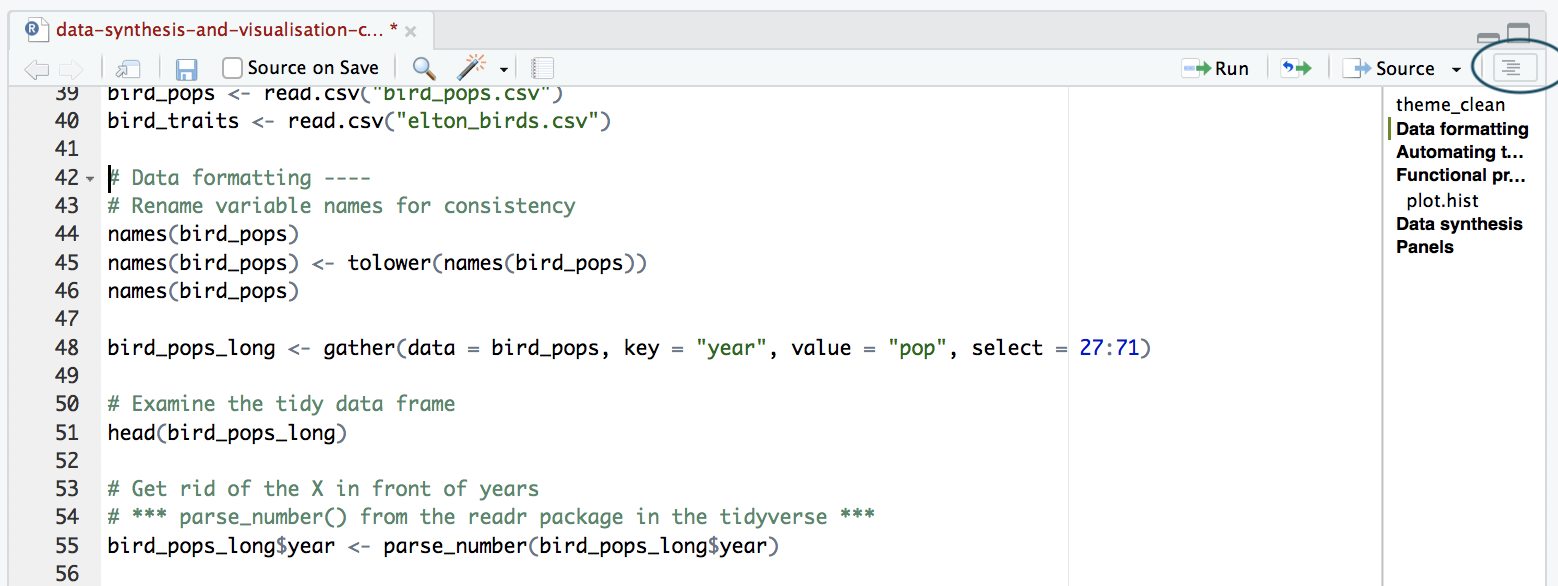
NOTE: If you don’t see the outline icon, you most likely do not have the newest version of RStudio - if you want to get this feature, you can download the newest version of RStudio.
Script structure:
There are no strict rules for the number and names of sections: you can adapt section content to your needs, but in general a script includes the following sections:
Introduction: Author statement (what does this script do?), author(s) names, contact details and date.
Libraries: What packages are you using for this script? Keep all of them together at the start of your script. When switching between scripts, with your packages already loaded, it’s easy to forget to copy across the library, which means future you might get confused as to why the code isn’t working anymore. Your library will be extra informative to you and other people if you add in comments about what you are using each package for. Here are two examples, good and bad, to illustrate these first two sections:
A not particularly useful script intro:
# My analysis
A more informative script intro:
# Analysing vertebrate population change based on the Living Planet Index
# Data available from http://www.livingplanetindex.org/

# Gergana Daskalova ourcodingclub(at)gmail.com
# 25-04-2017

# Libraries ----
library(tidyr)  # Formatting data for analysis
library(dplyr)  # Manipulating data
library(ggplot2)  # Visualising results
library(readr)  # Manipulating data
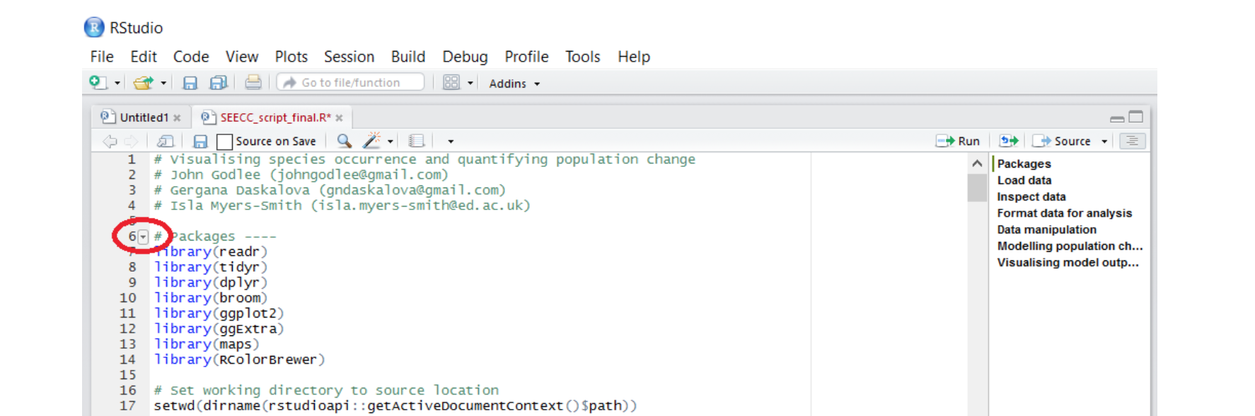
You might have noticed that when you create a section using four or more - at the end of a comment line, a little arrow appears in the margin next to the comment. Clicking these arrows allows you to collapse the section, which is very useful when traversing a long script.
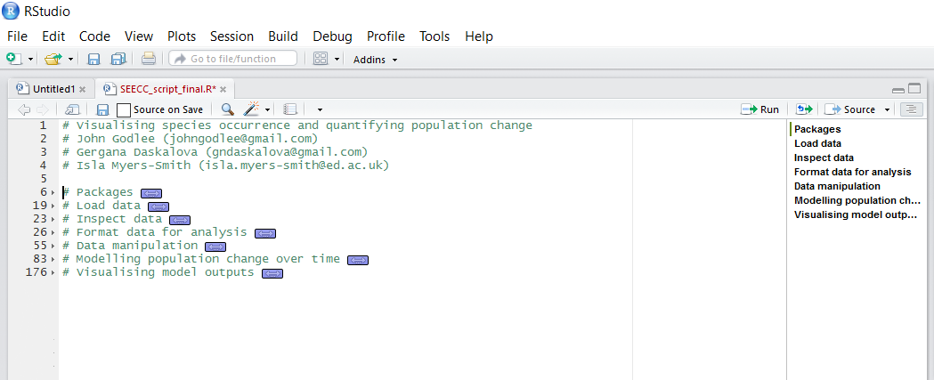
You can also go to Edit/Folding/Collapse all to collapse all sections. This is the outline of your script and from here you can navigate to whichever section you need. Expand all displays all of the code you’ve written. Here is an example:
Functions: Are you using any functions written by you and/or others? Define them here. For example, functions to remove NA values, functions to create your own ggplot2 theme. Here is an example functions section:
# Defining functions ----
# A custom ggplot2 function
theme.LPI <- function(){
  theme_bw()+
    theme(axis.text.x=element_text(size=12, angle=45, vjust=1, hjust=1),
          axis.text.y=element_text(size=12),
          axis.title.x=element_text(size=14, face="plain"),
          axis.title.y=element_text(size=14, face="plain"),
          panel.grid.major.x=element_blank(),
          panel.grid.minor.x=element_blank(),
          panel.grid.minor.y=element_blank(),
          panel.grid.major.y=element_blank(),
          plot.margin = unit(c(0.5, 0.5, 0.5, 0.5), units = , "cm"),
          plot.title = element_text(size=20, vjust=1, hjust=0.5),
          legend.text = element_text(size=12, face="italic"),
          legend.title = element_blank(),
          legend.position=c(0.9, 0.9))
}
If you run the code for the ggplot2 theme function above, you will see the name of the function you created appear in your Global Environment in the top right corner of your RStudio screen (you might need to scroll down past any objects you’ve created). Once you create a certain function, RStudio will remember it for the remainder of your session. If you close RStudio and then open it again later, you will need to run the code for the function again. NOTE: When you close RStudio, a message will ask if you want to save your workspace image. If you click yes, the next time you open RStudio, it will look exactly as it did when you closed it, with the same objects stored in your Global environment. If you click no, the next time you open RStudio, you will need to open your script and run through the code again if you want to use the same objects. We personally don’t often save our workspace image, as it makes RStudio run more slowly and can introduce errors as you might confuse objects from different analyses and/or overwrite objects without noticing.
Setting the working directory: It helps to keep all your data, scripts, image outputs etc. in a single folder. This minimises the chance of losing any part of your analysis and makes it easier to move the analysis on your computer without breaking filepaths. Note that filepaths are defined differently on Mac/Linux and Windows machines. On a Mac/Linux machine, user files are found in the ‘home’ directory (~), whereas on a Windows machine, files can be placed in multiple ‘drives’ (e.g. D:). Also note that on a Windows machine, if you copy and paste a filepath from Windows Explorer into RStudio, it will appear with backslashes (\ ), but R requires all filepaths to be written using forward-slashes (/), so you will have to change those manually. Set your working directory to the folder you downloaded from Github earlier, it should be called CC-etiquette-master. See below for some examples for both Windows and Mac/Linux:
# Set the working directory on Windows ----
setwd("D:/Work/coding_club/CC-etiquette-master")

# Set the working directory on Mac/Linux ----
setwd("~/Work/coding_club/CC-etiquette-master")
Importing data: what data are you using and where is it stored? Import LPIdata_CC.csv from your working directory. Here is an example:
# Import data ----
LPI <- read.csv("LPIdata_CC.csv")
The different sections of your analysis: what is the logical workflow of your analysis? Keep the order in which you tackle your analysis consistent. If this is code for an undergraduate dissertation, a thesis chapter, or a manuscript, you can follow the same order in your script. Here is an example. If you copy these across to a script file, you’ll see the sections appear. Once you have imported in LPIdata_CC.csv, run the following code to generate the plot called barplot, which you can see in the image below:
# Formatting data ----
LPI2 <- gather(LPI, "year", "abundance", 9:53)  # Transforming the data from wide to long format, some blank cells may disappear
	# gather function requires tidyr package
LPI2$year <- parse_number(LPI2$year)  # Do you see awkward Xs before all the years? This gets rid of them.
names(LPI2)  # Check what the different variables are called
names(LPI2) <- tolower(names(LPI2))  # Make all variable names lower case

# When manipulating data it's always good check if the variables have stayed how we want them
# Use the str() function
str(LPI2)

# Abundance is a character variable, when it should be numeric, let's fix that
LPI2$abundance <- as.numeric(LPI2$abundance)

# Calc summary stats for each biome in the LPI database ----
levels(LPI2$biome)  # list all biomes

LPI_biome_summ <- LPI2 %>%  # use of pipe operator
  group_by(biome) %>%  # Group by biome
  summarise(populations = n())  # Create columns, number of populations

# Visualising the number of populations in each biome with ggplot2 package ----
(barplot <- ggplot(LPI_biome_summ, aes(biome, color = biome, y = populations)) + geom_bar(stat = "identity") +
  		theme.LPI() +                     # Use of personal theme function
  		ylab("Number of populations") +
  		xlab("Biome") +
		theme(legend.position = "none"))  # Removal of legend for simplicity
Note that putting your entire ggplot code in brackets () creates the graph and then shows it in the plot viewer. If you don’t have the brackets, you’ve only created the object, but haven’t visualized it. You would then have to call the object such that it will be displayed by just typing barplot after you’ve created the “barplot” object.
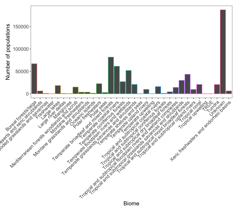 Figure 1. Abundance of species populations for each biome.
The outputs of your analysis: Remember to keep your filepath sensible not only when loading data in, but also when you are outputting files (e.g. .Rdata, .csv files and any figures you want saved). .csv files are more transferable and can be used across multiple platforms, whereas .Rdata files are more compressed and are quicker to work with. Saving graphs as .pdf files is better practice, since .pdf files are vector based and don’t decrease in quality when you zoom in or out. .png files, on the other hand, are easily inserted in text documents and presentations, so ideally you should save a .pdf and a .png file of your graph. It is also good practice to save image outputs in a subdirectory of your working directory, e.g. img/. Remember that you will have to create the folder img manually before saving plots to it:
png(file="img/biome_pop.png", width = 1000, height = 2000)  # Note that png() uses pixel values for width and height
ggplot(LPI_biome_summ, aes(biome, color = biome, y = populations)) + geom_bar(stat = "identity") +
  		theme.LPI() +
  		ylab("Number of populations") +
  		xlab("Biome") +
		theme(legend.position = "none")
dev.off()  # This tells R you are done with the plotting and it can save the file

pdf(file="img/biome_pop.pdf",  width = 13.33, height = 26.66)  # pdf() uses inches
ggplot(LPI_biome_summ, aes(biome, color = biome, y = populations)) + geom_bar(stat = "identity") +
  		theme.LPI() +
  		ylab("Number of populations") +
  		xlab("Biome") +
		theme(legend.position = "none")
dev.off()
Note that you can also save the outputs of your analysis with the use of another package ggsave, and you can refer to the end of this data visualization tutorial for an example of how to do so.
2. Following a coding syntax etiquette
2.1. Naming files and objects.
“There are only two hard things in Computer Science: cache invalidation and naming things.” - Phil Karlton
We’re not too familiar with cache invalidation, but we would definitely agree that naming things is hard and going for a quick and easy solution, like calling your graphs graph, might cause trouble later!
File names for scripts should be meaningful and end in .R. Avoid spaces and funky characters!!! They can cause trouble when uploading files to Github and in general when trying to locate files through certain file paths.
LPI_analysis_Apr_2017.R  # Alright.

yet_another_script.R  # Bad. Took me hours to find the file when I needed it one year later.
Object names should be concise and meaningful.
Calling your objects data or something similarly vague might cause problems if you are doing multiple analyses at once/don’t clean your environment periodically, as these object names will get overwritten and can mess up your script if you aren’t running it in order.
Long object names are annoying to type. More letters = higher chance you’ll make a typo.
Object, variable (e.g.object$variable) and function names should be lowercase. MinPrecip_august is confusing to remember, min.precip.aug is a bit long, but informative and easier to type.
- Variable names should be nouns. e.g.
abundancerichness - Function names should be verbs. e.g.
calc.sp.richness - Use an underscore to separate words within a script file. e.g.
LPI_analysis_Apr_2017.R - The preferred form for object/variable names is all lower case letters and words separated with underscores e.g. (
object_name$variable_name). - For functions, all lower case letters and words separated by dots e.g. (
function.name).
This way it is clear what is an object and what is an external file. These are not strict rules - variable names like variable_name are also acceptable. The most important thing is to be consistent: choose one style of variable, object and file names and stick with it!
# Object names
 avg_clicks  # Good.
 avg.clicks  # Acceptable.
 avg_Clicks  # Not okay.

# Function names
 calculate.avg.clicks  # This is what we are aiming for.
 CalculateAvgClicks  # Not that bad, but mixing capital and lowercase letters can lead to typos
 calculate_avg_clicks , calculateAvgClicks  # Bad. The convention is that functions are defined using dots, not underscores.
2.2 Spacing
Place spaces around all infix operators (=, +, -, <-, etc.). The same rule applies when using = in function calls.
Always put a space after a comma, and never before, just like in normal prose.
There are two exceptions to this rule (that we know of): : and :: don’t need spaces around them and one should not add spaces when defining coordinate systems in spatial objects.
x <- 1:10  # Good
base::get  # Good
dplyr::select  # When you use `package_name::function_name` in your code like the example here, this means you are calling the function `select()` from the package `dplyr` - this way of using functions works without having loaded the package beforehand using `library(dplyr)`, but it's not very commonly used, since it's longer.

crs.geo <- CRS("+proj=longlat +ellps=WGS84 +datum=WGS84")  # geographical, datum WGS84
# Here we are creating an imaginary object with a geographical projection commonly used for the UK
Don’t place a space before left parentheses, except in a function call.
# Good
if (debug) do(x)
plot(x, y)

# Bad
if(debug)do(x)
plot (x, y)
Extra spacing (i.e., more than one space in a row) is ok if it improves alignment of equal signs or assignments (<-).
# Sample code just to illustrate the point, no need to run the code at this point!
LPI_biome_summ <- LPI_long %>%
  group_by(biome) %>%  # Group by biome
  summarise(populations = n(),   # Create columns, number of populations
            mean_study_length_years = mean(lengthyear),  # mean study length
            max_lat = max(decimal_latitude),  # max latitude
            min_lat = min(decimal_latitude),  # max longitude
            dominant_sampling_method = names(which.max(table(sampling_method))),  # modal sampling method
            dominant_units = names(which.max(table(units))))  # modal unit type
Do not place spaces around code in parentheses or square brackets (unless there’s a comma, in which case see above).
# Good
if (debug) do(x)
diamonds[5, ]

# Bad
if ( debug ) do(x)  # No spaces around debug
x[1,]   # Needs a space after the comma
x[1 ,]  # Space goes after comma not before
Inline commenting: If you are commenting inline with code, place two spaces after the code, followed by #, a single space and then your text, e.g. summary(model)<space><space>#<space>comment.
# Calculating summary statistics for each biome in the Living Planet Index database
# No need to copy and run this code now, this just illustrates comments
LPI_biome_summ <- LPI2 %>%
  group_by(biome) %>%  # Group by biome
  summarise(populations = n(),   # Create columns, number of populations
            mean_study_length_years = mean(lengthyear),  # mean study length
            max_lat = max(decimal_latitude),  # max latitude
            min_lat = min(decimal_latitude),  # max longitude
            dominant_sampling_method = names(which.max(table(sampling_method))),  # modal sampling method
            dominant_units = names(which.max(table(units))))  # modal unit type
2.3 Curly braces
An opening curly brace should never go on its own line and should always be followed by a new line. A closing curly brace should always go on its own line, unless it’s followed by else.
Always indent the code inside curly braces.
# Good

if (y < 0 && debug) {
  message("Y is negative")
}

if (y == 0) {
  log(x)
} else {
  y ^ x
}

# Bad

if (y < 0 && debug)
{message("Y is negative")}

if (y == 0) {
  log(x)
}
else {
  y ^ x
}
It’s ok to leave very short statements on the same line:
if (y < 0 && debug) message("Y is negative")
2.4 Line length
The official convention is to limit your code to 80 characters per line. Having to continuously scroll left and right can be annoying and confusing. Also, when you publish your code to Github, the scroll bar is all the way down at the bottom of the page, so to scroll right, you first need to scroll all the way down, scroll right, then scroll all the way up to wherever you want to be … unnecessary.
How do you know what’s 80 characters though? RStudio can place a handy line in your editor as a reminder! Go to Tools/Global Options/Code/Display/Show Margin/80 characters. Sometimes it might make more sense for your code to be a bit longer than 80 characters, but in general code is easier to read if there is no need for continuous scrolling left and right: around 100 characters should work alright.
When using pipes from the dplyr package, keep the pipe operator %>% at the end of the line and continue your pipe on a new line.
# Just an example of what a pipe could look like, no need to run the code at this stage.
LPI_long <- LPI_long %>%
  group_by(., genus_species_id) %>%  # group rows so that each group is one population
  mutate(., maxyear = max(year), minyear = min(year)) %>%  # Create columns for the first and most recent years that data was collected
  mutate(., lengthyear = maxyear-minyear) %>%  # Create a column for the length of time data available
  mutate(., scalepop = (pop-min(pop))/(max(pop)-min(pop))) %>%  # Scale population trend data
  filter(., is.finite(scalepop)) %>%
  filter(., lengthyear > 5) %>%  # Only keep rows with more than 5 years of data
  ungroup(.)  # Remove any groupings you've greated in the pipe, not entirely necessary but it's better to be safe
When using ggplot2, keep the + at the end of the line and continue adding on layers on a new line.
# Just an example of what the code could look like, no need to run the code at this stage.
(vulture_scatter <- ggplot(vultureITCR, aes (x = year, y = abundance, colour = Country.list)) +
    geom_point(size = 2) +
    geom_smooth(method = lm, aes(fill = Country.list)) +
    theme_my_own() +
    scale_fill_manual(values = c("#EE7600", "#00868B")) +
    scale_colour_manual(values = c("#EE7600", "#00868B"),
                        labels = c("Croatia", "Italy")) +
    ylab("Griffon vulture abundance\n") +
    xlab("\nYear"))
2.5 Indentation
If a command runs over multiple lines, indent the second line to where the definition starts. You can check out the indentation in the ggplot2 code above: when you click Enter after the + sign, the new line automatically gets indented.
Here is a before and after of a ggplot2 figure code:
# Again, just an example, don't run this, it won't work!
ggplot()+geom_hline(yintercept=0,linetype="dotted",colour="darkgrey")+
  geom_line(data=cwa.sub, aes(x=Season,y=Total.Concentration),size=2,alpha=0.2)+
  geom_ribbon(data=preds2, aes(x=Season, ymin=ploBT, ymax=phiBT), fill="#3cd0ea", alpha=0.3)+
  geom_line(data=preds2,aes(x=Season,y=Total.ConcentrationBT),colour="#3cd0ea",size=3)+theme_bw()+ylab("Minimum Sea Ice Concentration")+xlab("Season")+annotate("text",x=2012,y=0.4,label=paste0("p = ",round(pval.cwa.sub,4)),size=6)+theme(legend.title=element_text(size=20,face="plain",hjust=1),legend.text=element_text(size=18,angle=45),legend.position="bottom",legend.key =element_blank(),axis.title.x=element_text(size=20,margin=margin(20,0,0,0)),axis.title.y=element_text(size=20,margin=margin(0,20,0,0)),axis.text=element_text(size=16),panel.grid.minor=element_blank(),panel.grid.major=element_blank())

(plot <- ggplot() +
  geom_hline(yintercept = 0, linetype = "dotted", colour = "darkgrey") +
  geom_line(data = cwa.sub, aes(x = Season, y = Total.Concentration), size = 2, alpha = 0.2) +
  geom_ribbon(data = preds2, aes(x = Season, ymin = ploBT, ymax = phiBT), fill = "#3cd0ea", alpha = 0.3) +
  geom_line(data = preds2, aes(x = Season, y = Total.ConcentrationBT), colour = "#3cd0ea", size = 3) +
  theme_bw() +
  labs(y = "Minimum Sea Ice Concentration", x = "Season") +
  annotate("text", x = 2012, y = 0.4, label = paste("p = ", round(pval.cwa.sub,4)), size = 6) +
  theme(legend.title = element_text(size = 20, face = "plain", hjust = 1),
        legend.text = element_text(size = 18, angle = 45),
        legend.position = "bottom",
        legend.key = element_blank(),
        axis.title.x = element_text(size = 20, margin = margin(20,0,0,0)),
        axis.title.y = element_text(size = 20, margin = margin(0,20,0,0)),
        axis.text = element_text(size=16),
        panel.grid.minor = element_blank(),
        panel.grid.major = element_blank()))

# The second version is much easier to read and there is no need to keep scrolling left and right.
3. Tidying up old scripts and data frames
It’s best to start following a sensible coding etiquette from the very beginning, but realistically we are often in a hurry: we want to code quickly and even if we know we are not following best practices, we still go ahead, because we are thinking of our short-term goals - getting it done, as opposed to the more long-term goals of having a sensible and reproducible record of our analysis. As we are writing this tutorial, we are just as guilty as everyone else of having messy scripts, missing spaces around =, etc. But it’s important to try to be consistent with your coding and once you get into the habit of it, it hopefully won’t seem like “one extra thing to do.”
What if you want to make your old code neater?
That’s a lot of spaces you might need to add in… First, you could try using RStudio to format the code for you. Click on Code/Reformat code and see what happens. You will get all the spaces in, but R puts the code on a new line after each comma - too many lines! You can try this instead (back up your scripts before you start any experimenting!!!):
# Reformat your old code to add in spaces and limit line length
install.packages("formatR")
library("formatR")

# Set working directory to wherever your messy script is
tidy_source("messy_script_2017-02-25.R", file = "tidy_script_2017-02-25.R", width.cutoff = 100)
# If you don't specify file = "new_script.R", your script will get overwritten, dangerous!
# If you don't specify a width cutoff point, tidy_source just adds in the spaces
# 100 characters seems like a reasonable cutoff point

# Reformat all the scripts in a directory
# Set your working directory to wherever your messy scripts are

# IMPORTANT this will override script files, so make a duplicate back up folder, in case tidy_dir messes up
tidy_dir(path="whatever/your/path/is", recursive = TRUE)
# recursive	- whether to look for R scripts in subdirectories of the directory specified under path
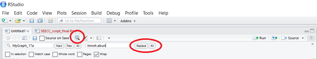
Renaming old objects and variables
If, like us, you find yourself having to use a script from before you knew any better, you might have objects with really uninformative, unnecesarily hard to type names. There is an easy fix to that: just like in most text editors, you can Find and Replace words, in our case object names. You can type up the object whose name you want to change, then add the new one and replace either individual occurrences, or all of the occasions when the object name is mentioned. You can also select lines of code and only rename the object in that part of the code - careful that you have clicked on In selection, as otherwise the object name will be replaced in the entire script, despite you having selected only some of the lines.
If you want to rename your variable names, that’s quickly done, too.
names(dataframe) <- gsub(".", "_", names(dataframe), fixed = TRUE)
# This code takes all of the variable names in the imaginary dataset `dataframe` and replaces `.` with `_`
# Depending on the naming style you are using, you might want to go the other way around and use `.` in all variable names

names(dataframe) <- tolower(names(dataframe))
# This code makes all of the variable names in the imaginary dataset lowercase

colnames(dataframe)[colnames(dataframe) == 'Old_Complicated_Name'] <- 'new.simple.name'
# Renaming an individual column in the imaginary dataset
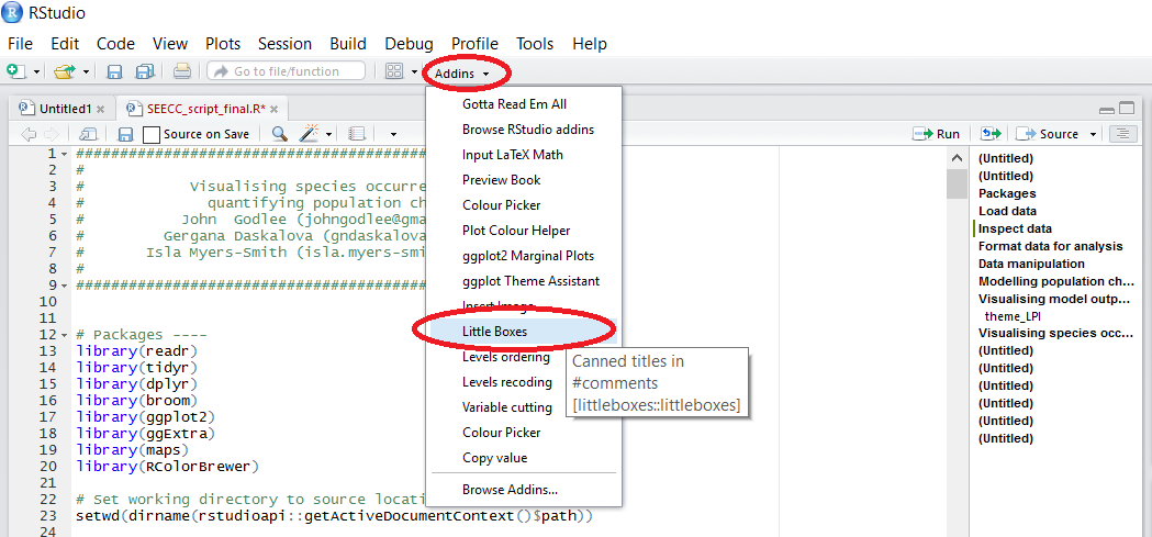
RStudio addins:
RStudio addins are available for the newest version of RStudio and add some functionality to RStudio using point and click menus. After you have installed certain addins, you can access them by clicking on Addins, which is under the Profile and Tools bar in the RStudio menu. To get a full list of RStudio plugins, run:
install.packages('addinslist')
When you click on Addins/Browse RStudio Addins, you will see the list of addins and the links to their Github repos.
Boxes around introductory sections of scripts have become a trendy addition to script files, definitely not an essential component, but if that appeals to you, you can add a box using this plugin, saving you the time of typing up many hashtags.
# Insert a box around the introductory section of your script
install.packages("devtools")
devtools::install_github("ThinkRstat/littleboxes")

# Afterwards select your introductory comments, click on Addins/ Little boxes and the box appears!
# Note that if you are also reformatting your code using formatR, reformat the code first, then add the box.
# formatR messes up these boxes otherwise!
Now that you have read through the tutorial, try to clean up bad_script.R, which can be found in the github repository for this tutorial, or tidy up one of your own scripts.
Our coding etiquette was developed with the help of Hadley Whickham’s R Style Guide.
Doing this tutorial as part of our Data Science for Ecologists and Environmental Scientists online course?
This tutorial is part of the Stats from Scratch stream from our online course. Go to the stream page to find out about the other tutorials part of this stream!
If you have already signed up for our course and you are ready to take the quiz, go to our quiz centre. Note that you need to sign up first before you can take the quiz. If you haven't heard about the course before and want to learn more about it, check out the course page.