Created by Declan V.

Welcome to this tutorial about data analysis with Python and the Pandas library. If you did the Introduction to Python tutorial, you’ll rememember we briefly looked at the pandas package as a way of quickly loading a .csv file to extract some data. This tutorial looks at pandas and the plotting package matplotlib in some more depth.

Tutorial aims:

Understand what Pandas is
Ways of running Python and Pandas
Understanding the basic Pandas data structures
Learn how to access data from a Pandas DataFrame
Learn how to filter data in a Pandas DataFrame
Learn how to read and sort data from a file
Understand the basics of the Matplotlib plotting package
Learn how to bring together other packages to enhance your plots
Learn how to further customise the appearance of Matplotlib plots
Be inspired to experiment further with Matplotlib!

1. What is Pandas?

pandas is a package commonly used to deal with data analysis. It simplifies the loading of data from external sources such as text files and databases, as well as providing ways of analysing and manipulating data once it is loaded into your computer. The features provided in pandas automate and simplify a lot of the common tasks that would take many lines of code to write in the basic Python langauge.

If you have used R’s dataframes before, or the numpy package in Python, you may find some similarities in the Python pandas package. But if not, don’t worry because this tutorial doesn’t assume any knowledge of NumPy or R, only basic-level Python.

Pandas is a hugely popular, and still growing, Python library used across a range of disciplines from environmental and climate science, through to social science, linguistics, biology, as well as a number of applications in industry such as data analytics, financial trading, and many others. In the Introduction to Python tutorial we had a look at how Python had grown rapidly in terms of users over the last decade or so, based on traffic to the StackOverflow question and answer site. A similar graph has been produced showing the growth of Pandas compared to some other Python software libraries! (Based on StackOverflow question views per month).

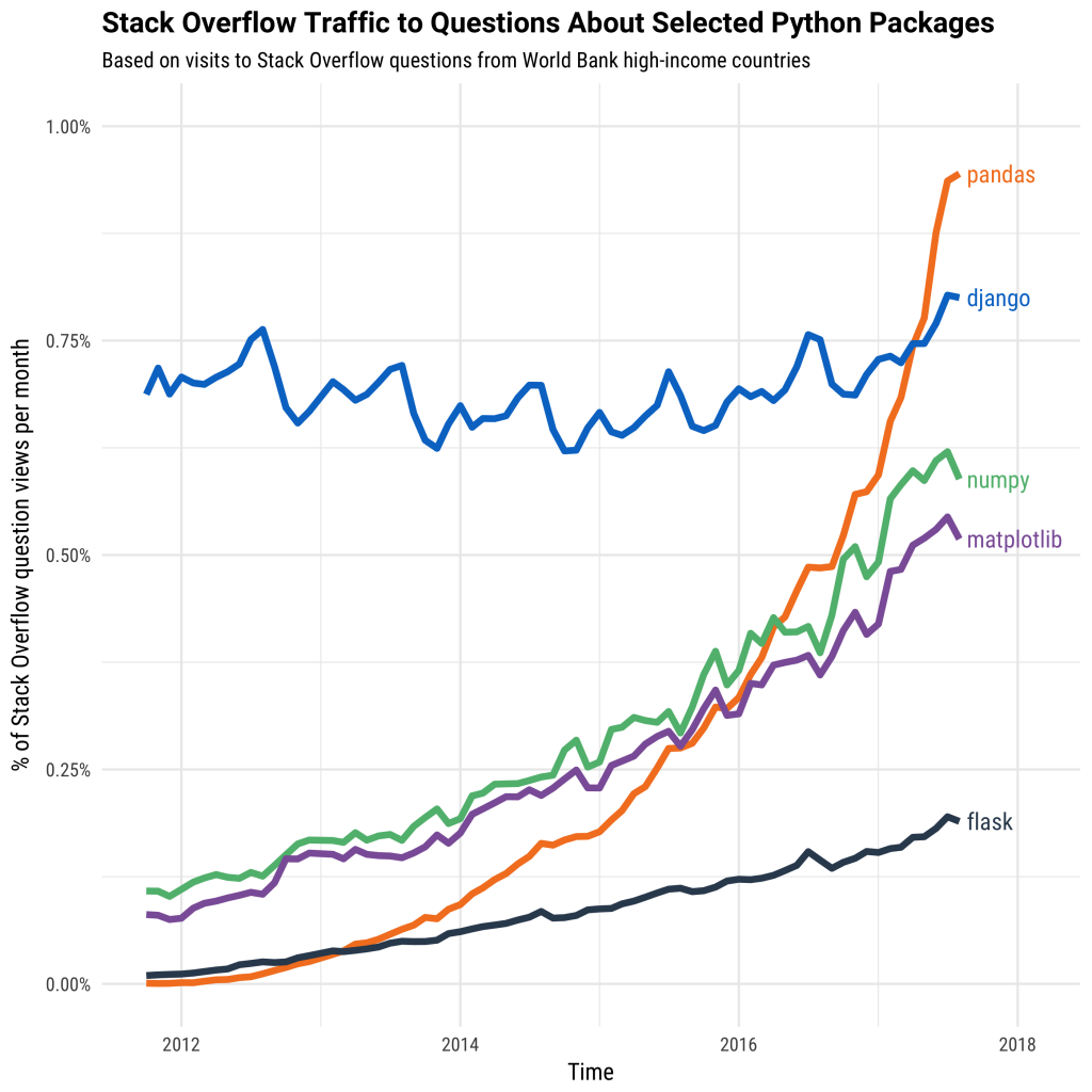
The growth of pandas vs other Python modules

These graphs of course should be taken with a pinch of salt, as there is no agreed way of absolutely determing programming langauge and library popularity, but they are interesting to think about nonetheless.

Pandas is best suited for structured, labelled data, in other words, tabular data, that has headings associated with each column of data. The official Pandas website describes Pandas’ data-handling strengths as:

Tabular data with heterogeneously-typed columns, as in an SQL table or Excel spreadsheet.
Ordered and unordered (not necessarily fixed-frequency) time series data.
Arbitrary matrix data (homogeneously typed or heterogeneous) with row and column labels.
Any other form of observational / statistical data sets. The data actually need not be labelled at all to be placed into a pandas data structure.

Some other important points to note about Pandas are:

Pandas is fast. Python sometimes gets a bad rap for being a bit slow compared to ‘compiled’ languages such as C and Fortran. But deep down in the internals of Pandas, it is actually written in C, and so processing large datasets is no problem for Pandas.
Pandas is a dependency of another library called statsmodels, making it an important part of the statistical computing ecosystem in Python.

You can read more about the Pandas package at the Pandas project website.

2. Ways of running Python with Pandas

Here we briefly discuss the different ways you can folow this tutorial. There are lots of different ways to run Python programs, and I don’t want to prescribe any one way as being the ‘best’. Users of RStudio and Matlab may find that the Spyder programming environment most closely matches the feel of RStudio and Matlab, with a window for editing scripts and an ‘interactive’ mode that can be used along side. For a more minimalist approach, you may prefer to write their scripts/programs in a text editor such as Notepadd++ (Windows), vim, emacs, or other popular editors. (But do not use Windows Notepad!). Personally this is how I like to work with Python as it frees you from the distractions of an IDE like Spyder, and reduces the number of problems that can arise from the Spyder program being set-up incorrectly.

Finally there is IPython, which lets you type in Python commands line-by-line, similar to Matlab and and RStudio, or an R console session.

Some more information on the three methods is described below:

Spyder

If you are attending the workshop ‘live’ on-site at Edinburgh University, the easiest way is to use the Spyder IDE (Integrated Development Environment) which is installed on the GeoSciences computers. It can also be installed on your laptop relatively easily. It is included in the Anconda Python distibution which can be downloaded here. Be sure to download the Python 3 version!

The basics of Spyder were covered in the Introduction to Python tutorial.

Text Editor with the Linux/Mac Terminal or Command-line

You can follow this tutorial by writing scripts saved as .py files and then running the script from the terminal or command line with the python command. e.g.

python myscript.py

(Although it looks simple, this way can quite tricky to set up with Windows, it is probably easiest on Linux or Mac.)

Interactively with IPython

IPython is an ‘interactive’ Python interpreter. It lets you type in Python commands line-by-line, and then immediately execute them. It’s a very useful way of quickly testing and exploring Python commands, because you don’t have to interact directly with the command line or run the entire script. Spyder has an IPython console built in to it (on the right hand panel), or it can be started in Linux/Mac from the command line by running:

ipython

Note for interactive (IPython) users: If you are following this tutorial with IPython, you do not need to use print functions to get IPython to display variables or other Python objects. IPython will automatically print out variable simply when you type in the variable name and press enter. So for example:

In [1]: my_var = "Hello, World!"

In [2]: my_var  # Now press ENTER
Out[2]: 'Hello, World!'

IPython users: When you see a print function used in this tutorial, e.g. print(my_var), you can omit it and simply type the variable name (e.g. my_var) and press ENTER.

On Windows you will find IPython in the start menu if it has been installed.

Conventions when using Pandas

All the examples in this tutorial assume you have installed the Python library pandas, either through installing a scientific Python distribution such as Anaconda, or by installing it using a package-manager, such as conda or pip. To use any of the features of Pandas, you will need to have an import statement at the top of your script like so:

import pandas as pd

By convention, the pandas module is almost always imported this way as pd. Every time we use a pandas feature thereafter, we can shorten what we type by just typing pd, such as pd.some_function().

If you are running Python interactively, such as in IPython, you will need to type in the same import statement at the start of each interactive session.

Try the following to see which version of Pandas you are running:

import pandas as pd

print(pd.__version__)

Reminder for IPython users: You do not need the print() function wrapped around the variable here. Just type pd.__version__ and press ENTER. Remember this every time you see a print function for the remainder of this tutorial.

Run the script and note the output. My script prints '0.22.0', but you may be on a slighty newer/older version of Pandas, which is OK for this introductory tutorial.

Files for this tutorial

This short tutorial is mainly based around working with the basic Pandas commands and data structures, but we also use some data about Scottish mountains, provided in the form of a .csv file (scottish_hills.csv).

You can download the data from this Github repository. Clone and download the repo as a zipfile by pressing the big green button, then unzip it. You should then save any Python scripts to that folder, so they can access the data easily.

Alternatively, you can fork the repository to your own Github account and then clone it using the HTTPS/SSH link. For more details on how to register on Github, download Git and use version control, please check out our previous tutorial.

The original data came from a series of databases about the mountains of Scotland, which if you are interested further can be found here: [http://www.haroldstreet.org.uk/other/excel-csv-files/].

As a side note, and some interesting trivia, the dataset we are using was originally compiled in 1891 by Sir Hugh Munro. He compiled a list of all the mountains in Scotland above 3000 feet (914m if you prefer the metric system). The table has been revised since with more accurate heights and coordinates.

3. Understand the basic Pandas data structures

Pandas has two core data structures used to store data: The Series and the DataFrame.

Series

The series is a one-dimensional array-like structure designed to hold a single array (or ‘column’) of data and an associated array of data labels, called an index. We can create a series to experiment with by simply passing a list of data, let’s use numbers in this example:

import pandas as pd

my_series = pd.Series([4.6, 2.1, -4.0, 3.0])
print(my_series)

The output should be:

  4.6
  2.1
 -4.0
  3.0
dtype: float64

Note that printing out our Series object prints out the values and the index numbers. If we just wanted the values, we can add to our script the following line:

print(my_series.values)

Which in addition will print:

array([ 4.6,  2.1, -4. ,  3. ])

For a lot of applications, a plain old Series is probably not a lot of use, but it is the core component of the Pandas workhorse, the DataFrame, so it’s useful to know about.

DataFrames

The DataFrame represents tabular data, a bit like a spreadsheet. DataFrames are organised into colums (each of which is a Series), and each column can store a single data-type, such as floating point numbers, strings, boolean values etc. DataFrames can be indexed by either their row or column names. (They are similar in many ways to R’s data.frame.)

We can create a DataFrame in Pandas from a Python dictionary, or by loading in a text file containing tabular data. First we are going to look at how to create one from a dictionary.

A refresher on the Dictionary data type

Dictionaries are a core Python data structure that contain a set of key:value pairs. If you imagine having a written language dictionary, say for English-Hungarian, and you wanted to know the Hungarian word for “spaceship”, you would look-up the English word (the dictionary key in Python) and the dictionary would give you the Hungarian translation (the dictionary value in Python). So the “key-value pair” would be 'spaceship': 'űrhajó'.

To construct a dictionary in Python, the syntax we would write is:

# Note that dictionaries are part of the core Python language
# You do not need 'import pandas' if you are only working with dictionaries.

hungarian_dictionary = {'spaceship': 'űrhajó'}

We could then look-up items in our dictionary with this syntax:

hungarian_dictionary['spaceship']

Dictionaries can have multiple entries (multiple key-value pairs), and these are separated with a comma:

hungarian_dictionary = {'spaceship': 'űrhajó',
                        'watermelon': 'görögdinnye',
                        'bicycle': 'kerékpár'}

The values in dictionaries are not limited to single strings or words. Values can be any Python object such as numbers, lists, tuples, or even other dictionaries:

# Names (keys) mapped to a tuple (the value) containing the height, lat and longitude.
scottish_hills = {'Ben Nevis': (1345, 56.79685, -5.003508),
                  'Ben Macdui': (1309, 57.070453, -3.668262),
                  'Braeriach': (1296, 57.078628, -3.728024),
                  'Cairn Toul': (1291, 57.054611, -3.71042),
                  'Sgòr an Lochain Uaine': (1258, 57.057999, -3.725416)}

Looking up a Scottish mountain using its name as the key would then give us the height, latitude and longitude as the value returned.

scottish_hills['Braeriach']

Enclosed in a print function, i.e. print(scottish_hills['Braeriach'], this would print out:

(1296, 57.078628, -3.728024)

Back to DataFrames…

If we didn’t have any real data to play with from an external file, we could manually create a DataFrame from a Python dictionary. Using the scottish_hills dictionary above, we can load it into a Pandas DataFrame with this syntax:

dataframe = pd.DataFrame(scottish_hills)

Note: You will sometimes see df used as shorthand convention for a DataFrame object in many Pandas examples, such as in the official Pandas documentation and on StackOverflow. (I have used dataframe for readability here.)

Try creating a Python script that converts a Python dictionary into a Pandas DataFrame, then print the DataFrame to screen. You can use the scottish_hills example or experiment with your own.

import pandas as pd

scottish_hills = {'Ben Nevis': (1345, 56.79685, -5.003508),
                  'Ben Macdui': (1309, 57.070453, -3.668262),
                  'Braeriach': (1296, 57.078628, -3.728024),
                  'Cairn Toul': (1291, 57.054611, -3.71042),
                  'Sgòr an Lochain Uaine': (1258, 57.057999, -3.725416)}

dataframe = pd.DataFrame(scottish_hills)
print(dataframe)

And the output should look like this:

    Ben Macdui    Ben Nevis    Braeriach   Cairn Toul  Sgòr an Lochain Uaine
1309.000000  1345.000000  1296.000000  1291.000000            1258.000000
  57.070453    56.796850    57.078628    57.054611              57.057999
  -3.668262    -5.003508    -3.728024    -3.710420              -3.725416

Now, this is not necessarily the most logical order to store data. It would probably make more sense for the columns to be categories or types of data, rather than the names of each hill. You may remember from previous workshops that the data is currently in wide format, but we want it in long format. To do this, we need to think about how to structure our dictionary. Pandas works best with dictionaries when the dictionary keys refer to column names or headers. Here’s a better dictionary to use:

scottish_hills = {'Hill Name': ['Ben Nevis', 'Ben Macdui', 'Braeriach', 'Cairn Toul', 'Sgòr an Lochain Uaine'],
                  'Height': [1345, 1309, 1296, 1291, 1258],
                  'Latitude': [56.79685, 57.070453, 57.078628, 57.054611, 57.057999],
                  'Longitude': [-5.003508, -3.668262, -3.728024, -3.71042, -3.725416]}

We’ve made the dictionary keys into category-like names, and then these are followed by a list of corresponding data values. Pandas will be able to read this better. Replace the dictionary in your script above and run it again. Now you should get the following output:

   Height   Latitude  Longitude              Hill Name
  1345  56.796850  -5.003508              Ben Nevis
  1309  57.070453  -3.668262             Ben Macdui
  1296  57.078628  -3.728024              Braeriach
  1291  57.054611  -3.710420             Cairn Toul
  1258  57.057999  -3.725416  Sgòr an Lochain Uaine

This is a more useful layout for our DataFrame. The column names are ordered alphabetically by default (left to right), but we can specify the order using the columns keyword. (Another way would be to use an OrderedDict data structure, but that’s not covered in this tutorial…)

In your original script, replace the line where you create the DataFrame with the following:

dataframe = pd.DataFrame(scottish_hills, columns=['Hill Name', 'Height', 'Latitude', 'Longitude'])

Run the modified script. You should now get output that looks like this:

               Hill Name  Height   Latitude  Longitude
            Ben Nevis    1345  56.796850  -5.003508
           Ben Macdui    1309  57.070453  -3.668262
            Braeriach    1296  57.078628  -3.728024
           Cairn Toul    1291  57.054611  -3.710420
Sgòr an Lochain Uaine    1258  57.057999  -3.725416

Note how the dictionary keys have become column headers running along the top, and as with the Series, an index number has been automatically generated. The columns are also in the order we specified.

4. Learn how to access data from a Pandas DataFrame

Pandas DataFrames have many useful methods that can be used to inspect the data and manipulate it. We are going to have a look at just a few of them.

If our DataFrame was huge, we would not want to print all of it to screen, instead we could have a look at the first n items with the head method, which takes the number of rows you want to view as its argument.

print(dataframe.head(3))

If we added this to the end of our script and ran it again, it would print:

    Hill Name  Height   Latitude  Longitude
 Ben Nevis    1345  56.796850  -5.003508
Ben Macdui    1309  57.070453  -3.668262
 Braeriach    1296  57.078628  -3.728024

We could also look at the last n rows with the tail method:

print(dataframe.tail(2))

Which would give us:

               Hill Name  Height   Latitude  Longitude
3             Cairn Toul    1291  57.054611  -3.710420
4  Sgòr an Lochain Uaine    1258  57.057999  -3.725416

Our columns in the dataframe object are individual Series of data. We can access them by referring to the column name e.g. dataframe['column-name']. Have a go at adding these extra statements to your script, and check that you get the same output:

print(dataframe['Hill Name'])

Should print:

              Ben Nevis
             Ben Macdui
              Braeriach
             Cairn Toul
  Sgòr an Lochain Uaine
Name: Hill Name, dtype: object

And:

print(dataframe['Height'])

Should print:

  1345
  1309
  1296
  1291
  1258
Name: Height, dtype: int64

Note that Pandas DataFrames are accessed primarily by columns. In a sense the row is less important to a DataFrame. For example, what do you think would happen using the following code?

dataframe[0]

(Try adding it your script somewhere at the end and printing the result.)

Ouch! That’s a lot of error messages… The columns cannot be accessed by their index number in this way, you must use the column name. You may have thought that this might return the row index instead, but we have to use a different method to get the row:

dataframe.iloc[0]

Gives you the row at position zero. (The “first” row in normal speech). This contains all the information about Ben Nevis:

Hill Name    Ben Nevis
Height            1345
Latitude       56.7968
Longitude     -5.00351
Name: 0, dtype: object

The iloc method gives us access to the DataFrame in more traditional ‘matrix’ style notation, i.e. [row, column] notation. So if we wanted to get the height of Ben Nevis specifically, we could do:

dataframe.iloc[0,0]

Which would give us 'Ben Nevis'.

A way to remeber this is that iloc is short for “integer location”. But a more Pandas-style approach would be to do:

dataframe['Hill Name'][0]

Which would also give us 'Ben Nevis'.

In other words, we are saying to our Pandas DataFrame “get me the Hill Name Series, and give me the zero-th item in that Series”. Remember Python uses zero-indexing (starts counting items from zero). Pandas is the same in this regard.

An even quicker way to access our columns (less typing) is to treat the names as if they were attributes of our DataFrame, like this:

dataframe.Height

This would return:

  1345
  1309
  1296
  1291
  1258
Name: Height, dtype: int64

Experiment with modifying your script (or interactively if using IPython) to access different elements of your DataFrame

5. Learn how to filter data in a Pandas DataFrame

We can also apply conditions to the data we are inspecting, such as to filter our data.

dataframe.Height > 1300

Would return:

   True
   True
  False
  False
  False
Name: Height, dtype: bool

This returns a new Series of True/False values though. To actually filter the data, we need to use this Series to mask our original DataFrame:

dataframe[dataframe.Height > 1300]

Learn how to append data to an existing DataFrame

We can also append data to the DataFrame. This is done using the following syntax:

dataframe['Region'] = ['Grampian', 'Cairngorm', 'Cairngorm', 'Cairngorm', 'Cairngorm']

Using the original script, try adding this line to the end of the script to append the Regions data and then printing the DataFrame again. If you are following the tutorial by building up a script as you go along, it should now look like this:

import pandas as pd

scottish_hills = {'Hill Name': ['Ben Nevis', 'Ben Macdui', 'Braeriach', 'Cairn Toul', 'Sgòr an Lochain Uaine'],
                  'Height': [1345, 1309, 1296, 1291, 1258],
                  'Latitude': [56.79685, 57.070453, 57.078628, 57.054611, 57.057999],
                  'Longitude': [-5.003508, -3.668262, -3.728024, -3.71042, -3.725416]}

dataframe = pd.DataFrame(scottish_hills, columns=['Hill Name', 'Height', 'Latitude', 'Longitude'])
dataframe['Region'] = ['Grampian', 'Cairngorm', 'Cairngorm', 'Cairngorm', 'Cairngorm']
print(dataframe)

Run the script again, the output should now be:

               Hill Name  Height   Latitude  Longitude     Region
            Ben Nevis    1345  56.796850  -5.003508   Grampian
           Ben Macdui    1309  57.070453  -3.668262  Cairngorm
            Braeriach    1296  57.078628  -3.728024  Cairngorm
           Cairn Toul    1291  57.054611  -3.710420  Cairngorm
Sgòr an Lochain Uaine    1258  57.057999  -3.725416  Cairngorm

6. Learn how to read data from a file using Pandas

So far we have only created data in Python itself, but Pandas has built in tools for reading data from a variety of external data formats, including Excel spreadsheets, raw text and .csv files. It can also interface with databases such as MySQL, but we are not going to cover databases in this tutorial.

We’ve provided the scottish_hills.csv file in this Github repository. The file contains all the mountains above 3000 feet (about 914 metres) in Scotland. We can load this easily into a DataFrame with the read_csv function.

If you are writing a complete script to follow the tutorial, create a new file and enter:

import pandas as pd

dataframe = pd.read_csv("scottish_hills.csv")
print(dataframe.head(10))

Run the script, and you should get the following output:

                    Hill Name  Height   Latitude  Longitude    Osgrid
     A' Bhuidheanach Bheag   936.0  56.870342  -4.199001  NN660775
             A' Chailleach   997.0  57.693800  -5.128715  NH136714
             A' Chailleach   929.2  57.109564  -4.179285  NH681041
A' Chraileag (A' Chralaig)  1120.0  57.184186  -5.154837  NH094147
           A' Ghlas-bheinn   918.0  57.255090  -5.303687  NH008231
             A' Mhaighdean   967.0  57.719644  -5.346720  NH007749
            A' Mharconaich   973.2  56.857002  -4.290668  NN604762
                Am Basteir   934.0  57.247931  -6.202982  NG465253
                 Am Bodach  1031.8  56.741727  -4.983393  NN176650
             Am Faochagach   953.0  57.771801  -4.853899  NH303793

We’ve used the head() function to give us only the first 10 items in the DataFrame, and avoid printing all 282 hills out to screen…

It looks like this table contains the hills in alphabetical order. It would be nice to see them in order of height. We can sort the DataFrame using the sort_values method. You can add the following lines to your script:

sorted_hills = dataframe.sort_values(by=['Height'], ascending=False)

# Let's have a look at the top 5 to check
print(sorted_hills.head(5))

Run the script with these extra lines, and have a look at the output:

                       Hill Name  Height   Latitude  Longitude    Osgrid
                   Ben Nevis  1344.5  56.796891  -5.003675  NN166712
 Ben Macdui (Beinn Macduibh)  1309.0  57.070368  -3.669099  NN988989
                  Braeriach  1296.0  57.078298  -3.728389  NN953999
                 Cairn Toul  1291.0  57.054397  -3.710773  NN963972
      Sgor an Lochain Uaine  1258.0  57.058369  -3.725797  NN954976

We now have our hills sorted by height. Note how we’ve used the by=['Height'] argument to specify that we want to sort by height, and then the ascending=False argument to get the heights sorted in descending order, from highest to lowest.

7. Understand the basics of the Matplotlib plotting package

matplotlib is a Python package used for data plotting and visualisation. It is a useful complement to Pandas, and like Pandas, is a very feature-rich library which can produce a large variety of plots, charts, maps, and other visualisations. It would be impossible to cover the entirety of Matplotlib in one tutorial, so this section is really to give you a flavour of the capabilities of Matplotlib, and to cover some of the basics, as well as a couple of more interesting ‘advanced’ features.

If you have a bit of basic Python knowledge already, the common route to learning Matplotib is to find examples of plots similar to ones you are trying to create and walk through them, trying to reproduce them with your own data perhaps. A great starting point is the Matplotlib gallery of examples. I recommend this because in practice it is difficult to cover each and every plot type, as the needs of scientists differ considerably depending on the type of data they are working with or the message they are trying to convey in their visualisation. You might also find it useful to refer to the Matplotlib official documentation as you go along.

Matplotlib conventions

Like Pandas, Matplotlib has a few conventions that you will see in the examples, and in resources on other websites such as StackOverflow. Typically, if we are going to work on some plotting, we would import matplotlib like this:

import matplotlib.pyplot as plt

And thereafter, we could access the most commonly used features of Matplotlib with plt as shorthand. Note that this import statement is at the submodule level. We are not importing the full matplotlib module, but a subset of it called pyplot. Pyplot contains the most useful features of Matplotlib with an interface that makes interactive-style plotting easier. Submodule imports have the form import module.submodule and you will see them used in other Python libraries too sometimes.

Matplotlib basics

We’re going to use the Scottish hill data from the Pandas section of the tutorial, so if you need to set this up again, the script should look like this to begin with:

import pandas as pd
import matplotlib.pyplot as plt

dataframe = pd.read_csv("scottish_hills.csv")

Let’s have a look at the relationship between two varibles in our Scottish hills data. Suppose I have a hypothesis that the height of Scottish hill increases with latitude northwards. Were going to plot height against latitude. To save typing later on, we can extract the Series for “Height” and “Latitude” by assigning each to a new variable, x and y, respectively.

Append the following to the script above:

x = dataframe.Height
y = dataframe.Latitude

(This saves us having to type dataframe.Height etc. every time)

Then we can plot them as a scatter chart by adding:

plt.scatter(x, y)

To make Python show the chart, we need to either save the figure, or show it in Spyder. To do this from the script add:

plt.show()

plt.savefig("my_chart_name.png")

Your script should look like this now:

import pandas as pd
import matplotlib.pyplot as plt

dataframe = pd.read_csv("scottish_hills.csv")
x = dataframe.Height
y = dataframe.Latitude
plt.scatter(x, y)
plt.show()  # or plt.savefig("name.png")

Run the script and have a look at the figure. It should look something like this:

Simple scatterplot

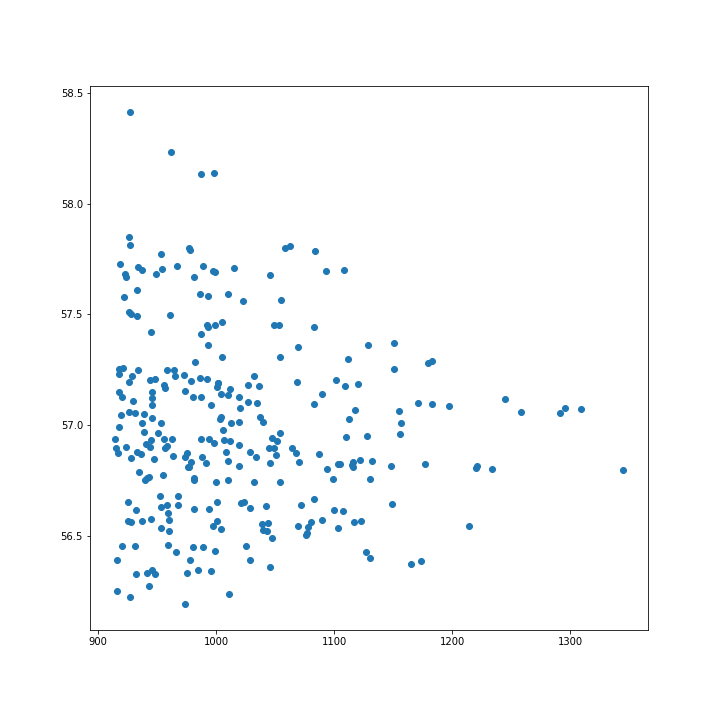
IPython users: the figure should render automatically after calling plt.scatter(x, y).

8. Learn how to bring together other Python libraries with Matplotlib

Now we are going to do some basic statistics so we can plot a line of linear regression on our chart. I’m a software engineer, not a statistician, so this will be pretty basic…

Let’s plot a linear regression through the data. Python has a library called scipy that contains a lot of statistics routines. We can import it by adding to the top of our script:

from scipy.stats import linregress

Then at the bottom of our script, we are going to get statistics for the linear regression by using a function called linregress by adding the following line. Don’t worry, we will go through below how all of this works. These are the lines you need to add to the end of your script:

stats = linregress(x, y)

m = stats.slope
b = stats.intercept

Let’s pause and recap what we’ve done here before plotting the regression.

We used an import statement with a slightly different format here: from module.submodule import function. This is a handy way of importing just a single function from a Python module. In this case we only want to use the linregress function in SciPy’s stats submodule, so we can just import it without anything else using that syntax.
Next we are assigning the results of linregress to variable called stats.
The linregress function is slightly different to the functions we’ve seen so far, because it returns an object with multiple values. In fact it returns the slope, intercept, rvalue, pvalue, and stderr (standard error). We can get hold of each of these values by using the dot notation: e.g. stats.slope, for example, much in the same way we can access our DataFrame attributes with dataframe.Height.
For ease of typing later, we’ve assigned the stats.slope to a variable m, and stats.intercept to a variable b.

The equation for the straight line that describes linear regression is y = mx + b, where m is the slope and b is the intercept.

Therefore, we can then plot the line of linear regression by adding the following line:

plt.plot(x, m * x + b)  # The equation of the straight line.

That’s a lot of new Python, so let’s review what the final script should look like:

import pandas as pd
import matplotlib.pyplot as plt
from scipy.stats import linregress

dataframe = pd.read_csv("scottish_hills.csv")

x = dataframe.Height
y = dataframe.Latitude

stats = linregress(x, y)

m = stats.slope
b = stats.intercept

plt.scatter(x, y)
plt.plot(x, m * x + b, color="red")   # I've added a color argument here

plt.savefig("figure.png")

# Or you can use plt.show()

Hopefully, you will have a figure that should look similar to this:

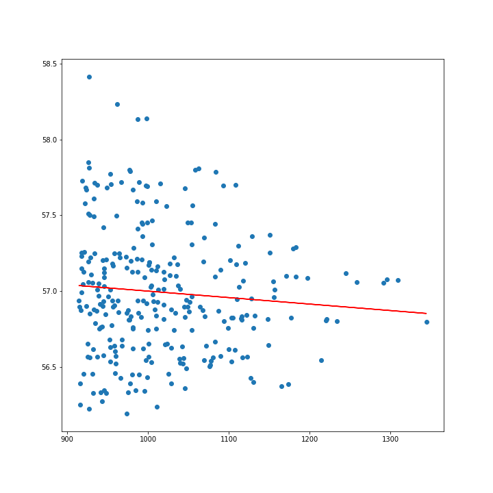
Scatterplot with linear regression line

I will leave it as an exercise for the reader to determine if they think this is a good fit or statistically significant…

(Hint: you have some extra information in the stats object - stats.rvalue and stats.pvalue.)

9. Learn how to customise Matplotlib plots further

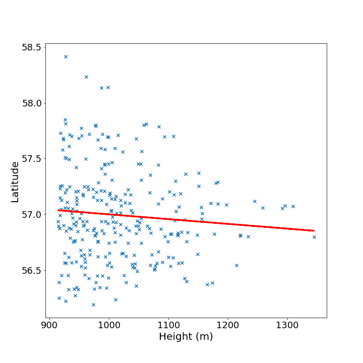
Matplotlib figures are highly customisable, and there are so many options it is usually best to consult the documentation first. In addition, the Matplotlib official pyplot tutorial is quite useful. To get started on Matplotlib plot customisation, here is an extended version of the above which sets the font sizes, axes lables, linewidths, and marker types:

Again, the best way to learn the features of Matplotlib is by example, so try to modify your script above with some of the extra arguments added below, such as fontsize, linewidth, color, etc. Have a go at adding your own values, and producing nicer looking plots. Here’s my example to start you off:

import pandas as pd
import matplotlib.pyplot as plt
from scipy.stats import linregress

dataframe = pd.read_csv("scottish_hills.csv")

x = dataframe.Height
y = dataframe.Latitude

stats = linregress(x, y)

m = stats.slope
b = stats.intercept

# Change the default figure size
plt.figure(figsize=(10,10))

# Change the default marker for the scatter from circles to x's
plt.scatter(x, y, marker='x')

# Set the linewidth on the regression line to 3px
plt.plot(x, m * x + b, color="red", linewidth=3)

# Add x and y lables, and set their font size
plt.xlabel("Height (m)", fontsize=20)
plt.ylabel("Latitude", fontsize=20)

# Set the font size of the number lables on the axes
plt.xticks(fontsize=18)
plt.yticks(fontsize=18)

plt.savefig("python-linear-reg-custom.png")

It will produce a figure that looks like this:

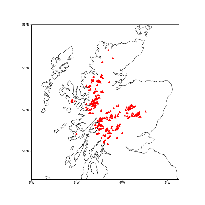
Scatter plot with cross point style

10. Bonus Matplotlib: plotting data onto maps with Cartopy

The best way to learn Matplotlib I believe is to learn from examples. I’m going to leave you with two examples that use an extra Python package called cartopy, unfortunately, Cartopy is not installed (yet) on the University of Edinburgh’s lab computers, so you will have to try this at home or on your own laptops later. We won’t go through this step-by-step in the tutorial, it is more of an example of how you could take things further in your own time.

The easiest way to install Cartopy on your own computer is with the package manager conda which you can access by typing into a terminal:

conda install -c conda-forge cartopy

This is only a short example, so don’t worry if you can’t install it right now, just try to follow the code and have look at the final figure.

import cartopy.crs as ccrs
from cartopy.mpl.ticker import LongitudeFormatter, LatitudeFormatter
import cartopy.feature as cfeature

plt.figure(figsize=(20,10))
ax = plt.axes(projection=ccrs.Mercator())
ax.coastlines('10m')

ax.xaxis.set_visible(True)
ax.yaxis.set_visible(True)

ax.set_yticks([56,57,58,59], crs=ccrs.PlateCarree())
ax.set_xticks([-8, -6, -4, -2], crs=ccrs.PlateCarree())

lon_formatter = LongitudeFormatter(zero_direction_label=True)
lat_formatter = LatitudeFormatter()

ax.xaxis.set_major_formatter(lon_formatter)
ax.yaxis.set_major_formatter(lat_formatter)

ax.set_extent([-8, -1.5, 55.3, 59])

plt.scatter(dataframe['Longitude'],dataframe['Latitude'],
                    color='red', marker='^', transform=ccrs.PlateCarree())
plt.savefig("munros.png")

Map of munros in Scotland

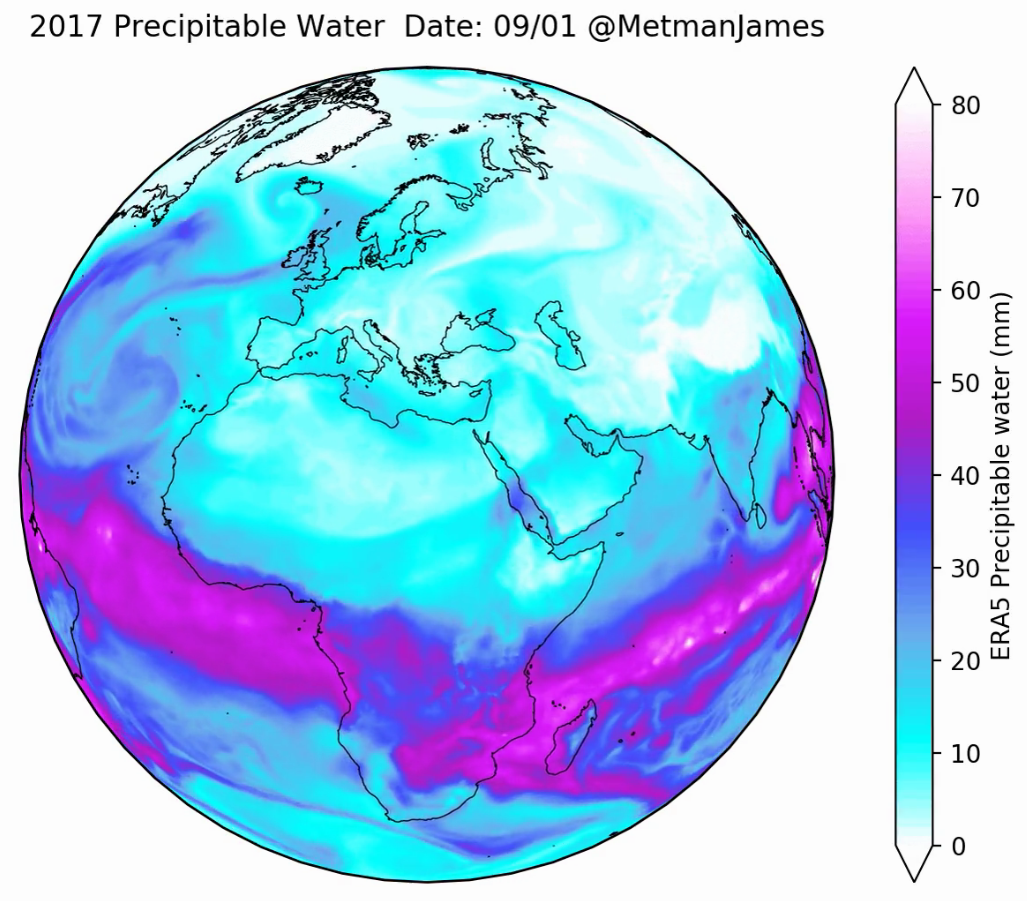
Finally, there is one more bonus Matplotlib example plot I would like to share, create by PhD student James Warner at Exeter University. It shows precipitable water in the atmopshere over the year 2017, projected over the globe. He has even created an animation of it which can be viewed on his Twitter account. This was all done using Python and some other Python libraries, including Matplotlib, Numpy, Cartopy, and a few others. It would take a long time to explain all of it, but hopefully it is some inspiration of the cool things you can do in Python with data visualisation.

The Python code for this is actually not too complicated and he has shared it here.

If you are feeling ambitious, try reproducing the images!

Global projection of precipitable water, 2017

Summary

In this tutorial we have covered the various ways in which we can use Pandas, Matplotlib, and a few other Python libraries to start doing data analysis.

Tutorial outcomes

Understood what the Pandas library does
Understood the basic Pandas data structures and how to manipulate them.
Understood the basics of the Matplotlib plotting package
Learnt how to bring use additional packages to enhance your plots

Python Data Analysis with Pandas and Matplotlib

Create plots and manipulate data with Pandas and Matplotlib