Tutorial Aims:
- Learn how to format survey data, coding responses, data types etc.
- Practise visualising ordinal data, count data, likert scales
- Mining text responses and comments for keywords
- Statistically analyse qualitative data
This workshop will explore qualitative data, the sort of data you might collect through responses to survey questions, interview transcripts, or observations. The data analysis techniques in this workshop lend themselves well to sociological research, and the examples we will use come from a study on human behaviour related to environmentally friendly actions, but they could easily be applied to observations of any system. For example, you might use an ordinal scale (e.g. 1-5, Disagree-Agree) to describe the perceived health of a plant seedling, with the question being something like “How wilted are the leaves? 1 = no sign of damage, 5 = leaves abcised”.
Firstly, we will learn how to format data from surveys and interviews effectively so that it can be easily used in analysis later. Then we will explore ways to visualise these data graphically. Finally, we will run some simple statistical analyses to answer some hypotheses.
ll the files you need to complete this tutorial can be downloaded from this repository. Please download the repo as a zip file (by clicking Code -> Download ZIP), then unzip it before starting the tutorial.
Alternatively, you can fork the repository to your own GitHub account and then add it as a new RStudio project by copying the HTTPS/SSH link. For more details on how to register on GitHub, download git, sync RStudio and GitHub and use version control, please check out our git and RStudio tutorial.
Getting Started
The first thing to do is open RStudio. Then make a new script file using File/ New File/ R Script, save it with a logical name inside the folder you just downloaded and unzipped from the Github repository.
Next, in your script file you need to set your working directory to the folder you just downloaded from the Github repository. Copy and paste the code below as a guide, but remember that the location of the folder on your computer will be different:
setwd("~/Downloads/CC-Qualit-master")
Next, load the packages needed for this tutorial by copying the code below into your script file then running those lines of code using either Cmd + Enter on a Mac, or Ctrl + Enter on Windows. If this is the first time you’re using them these packages, you’ll need to install them first, for example using install.packages("tidyverse"), and afterwards you can use library() to load them.
library(tidyverse)
library(RColorBrewer)
library(tidytext)
library(R.utils)
library(wordcloud)
library(viridis)
Finally, load the data files we will be using for the tutorial.
# The survey responses
sust_data <- read_csv("sust_behaviour.csv")

# A lookup table which connects each column in `sust_data` to the actual question on the survey
sust_lookup <- read_csv("sust_lookup.csv")

# A list of boring and non-useful words, bundled with `tidytext`
data(stop_words)
These are anonymised data from an online survey designed to investigate whether gender and different cohabitation arrangements influence the likelihood of participants performing environmentally friendly actions around the house, like recycling or buying sustainable household products.
This example dataset is formatted to purposely resemble the sort of thing you might generate from your own survey responses on Google Forms or Survey Monkey. It is not quite ready for analysis yet. We will spend some time getting the data ready for analysis, so that you can learn the skills needed to format your own data for analysis.
The object sust_lookup is a table which connects the name of each column in the dataframe to the corresponding question that was asked in the survey. Replacing the raw questions with shorter column names makes it much easier to write code, and with the lookup table we can add the actual question title back in when we are creating plots.
1. Formatting qualitative data
Getting qualitative data into a suitable format for analysis is a key pre-requisite for success - you’re setting yourself up for the coding fun to follow! Most analytical tools are best suited to numerical datasets, so some coercion is needed to generate numerical values from our qualitative observations. When you are designing a survey, emember to consider how you will analyse the data, draw out how you imagine your graphs will look, etc., this will make it much easier later on.
Some of the questions in this data set were designed on a five point scale, also known as a Likert scale. Each column in the dataframe contains responses to a single question. You can Look at the values contained in the column titled sustainability_daily_think entering this code:
unique(sust_data$sustainability_daily_think)
You should see that the column contains five discrete categories that follow an intuitive order from low to high: Never, Rarely, Sometimes, Often, All the time . We could just treat the responses as factors, but this doesn’t take into account their ordinal nature, any plots that we make will simply place the factors in alphabetical order, so instead we will ask R to treat them as an “ordered factor” using this code:
sust_data$sustainability_daily_think <- factor(sust_data$sustainability_daily_think,
	levels = c("Never", "Rarely", "Sometimes", "Often", "All the time"),
	ordered = TRUE)
Look for other columns that you think contain ordered factor data like these ones, then change them to ordered factors in the same way you did above. You can search for columns using:
head(sust_data)
OR
glimpse(sust_data)
Other columns in the data frame, such as sust_data$energy_action, contain strings of letters, e.g. BDEFH. This question on the survey presented the user with a list of sustainable actions related to the home, e.g. “I have replaced my lightbulbs with energy saving lightbulbs” and asked the user to tick all the ones that applied to them. Each of the letters refers to a single action. The format of this column is similar to what you would receive if you downloaded the raw results of a Google Form.
Imagine we want to ask the question “Does the number of sustainable energy-related actions performed vary according to gender?”. To do this we need to create a column in the data frame which counts the number of letters in sust_data$energy_action. To do this we can use nchar(), a simple function which counts the number of characters in a string. Additionally, we have to use as.character() to coerce energy_action to a character variable, as it is currently encoded as a factor, which isn’t compatible with nchar().
:
sust_data$energy_action_n <- nchar(as.character(sust_data$energy_action))
2. Visualising qualitative data
Now that we formatted our data for analysis we can visualise the data to identify interesting patterns.
Let’s start with the Likert scales. We can create bar charts to visualise the number of responses to a question which fit into each of the ordinal categories. The correct form for the bar chart will depend on the type of question that was asked, and the wording of the various responses. For example, if potential responses were presented as “Strongly disagree”, “Disagree”, “Neither agree nor disagree”, “Agree”, “Strongly agree”, you could assume that the neutral or zero answer is in the middle, with Disagree being negative and Agree being positive. On the other hand, if the answers were presented as “Never”, “Rarely”, “Sometimes”, “Often”, “All the time”, the neutral or zero answer would be Never, with all other answers being positive. For the first example, we could use a “diverging stacked bar chart”, and for the latter we would just use a standard “stacked bar chart”.
Diverging stacked bar chart
Let’s first make a diverging stacked bar chart of responses to the question: “How often during a normal day do you think about the sustainability of your actions?”. Investigating how gender affects the response. You can see from the lookup table (sust_lookup) that the responses to this question are stored in the column called sustainability_daily_think.
Check for yourself by entering the code below to display the contents of the sust_lookup object:
sust_lookup
If you look in the sustainability_daily_think column, you will see that it contains rows like Often, Never, and All the time:
sust_data$sustainability_daily_think
First, we need to make a summary data frame of the responses from this column, which can be done easily using the dplyr package. For an introduction to dplyr, check out our tutorial on data manipulation and formatting. You can use the code below to make a summary table:
sust_think_summ_wide <- sust_data %>%
	group_by(gender, sustainability_daily_think) %>%  # grouping by these two variables
	tally() %>%  # counting the number of responses
	mutate(perc = n / sum(n) * 100) %>%
	dplyr::select(-n) %>%
	group_by(gender) %>%
	spread(sustainability_daily_think, perc)
group_by() and tally() work together to count the number of responses to the question, splitting the count into each combination of gender (e.g. Male, Female) and type of response (e.g. Never, Often, etc.). mutate() creates another column called perc which is the percentage of the total respondents which responded based on their gender and response. dplyr::select() drops the n column which was created using tally(). The second group_by() and spread() work together to convert the data frame from long format, to wide format. It’s easier to demonstrate what this means with a diagram:
Long Format:
| gender | sustainability_daily_think | perc | |
|---|---|---|---|
| 1 | Female | Never | 1.575 |
| 2 | Female | Rarely | 1.575 |
| 3 | Female | Sometimes | 32.283 |
| 4 | Female | Often | 51.181 |
| 5 | Female | All the time | 13.386 |
| 6 | Male | Never | 3.125 |
| 7 | Male | Rarely | 6.250 |
| 8 | Male | Sometimes | 34.375 |
| 9 | Male | Often | 37.500 |
| 10 | Male | All the time | 18.750 |
Wide Format:
| gender | Never | Rarely | Sometimes | Often | All the time | |
|---|---|---|---|---|---|---|
| 1 | Female | 1.575 | 1.575 | 32.283 | 51.181 | 13.386 |
| 2 | Male | 3.125 | 6.250 | 34.375 | 37.500 | 18.750 |
In a long format, each column contains a unique variable (e.g. gender, percentage), whereas in a wide format, the percentage data is spread across five columns, where each column is a response type.
And now for the code to create the plot. First, let’s have a look at what we are aiming for:
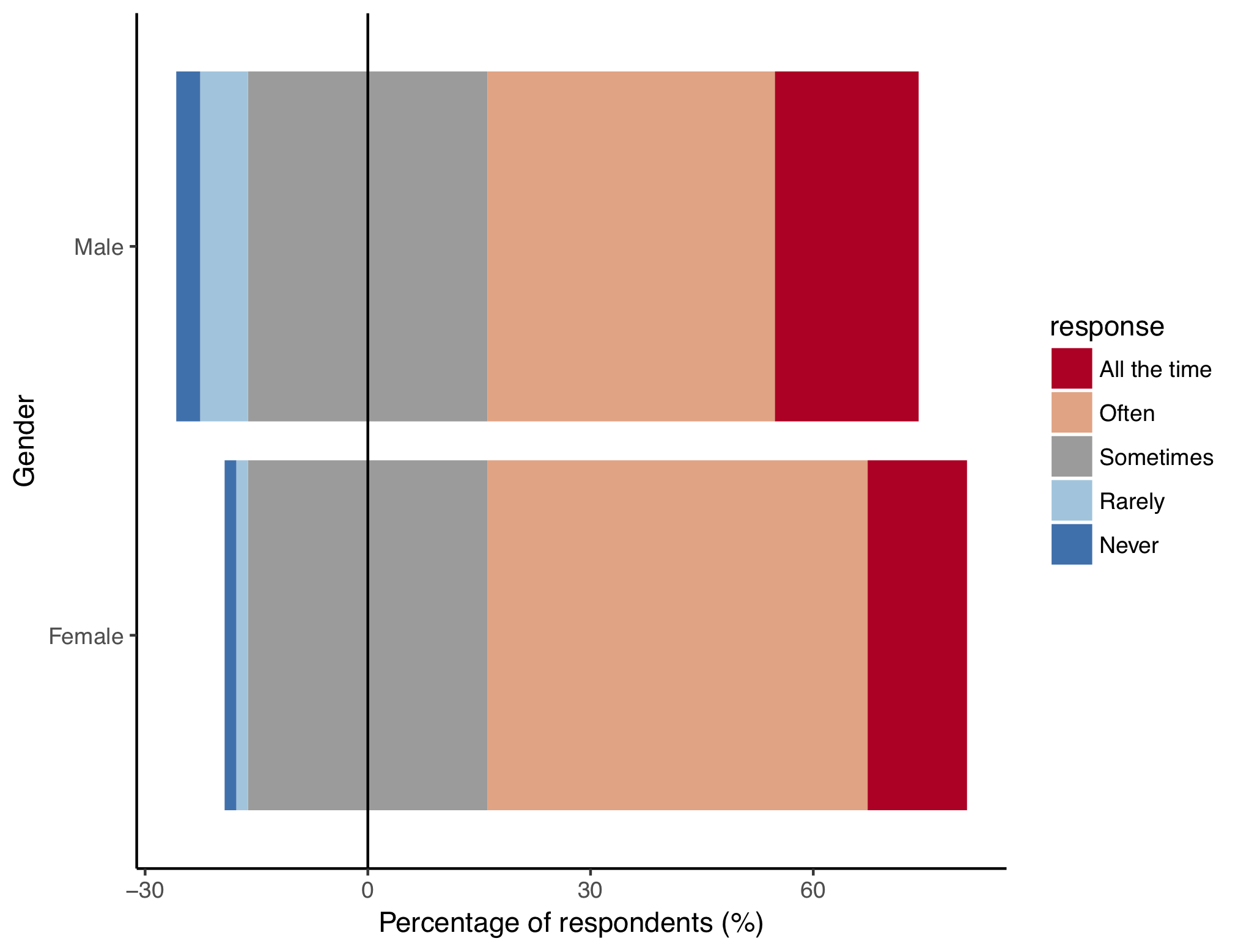
This type of plot is called a diverging stacked bar chart. “Stacked” means that each bar is further split into sub-categories, in this case each bar is a gender and each sub-bar is the percentage of that gender giving a particular response. “Diverging” means that the bar is straddled over the zero line. Formatting the bar chart in this way allows us to make a visual distinction between negative responses (i.e. Never, Rarely), positive responses (i.e. Often, All the time) and neutral responses (i.e. Sometimes).
To get the “Sometimes” responses to straddle the 0 line, we have to split the “Sometimes” values into two groups (midlow and midhigh), one group will sit below the zero line and one group will sit above. To do this we can use dplyr again:
sust_think_summ_hi_lo <- sust_think_summ_wide %>%
	mutate(midlow = Sometimes / 2,
		midhigh = Sometimes / 2) %>%
	dplyr::select(gender, Never, Rarely, midlow, midhigh, Often, `All the time`) %>%
	gather(key = response, value = perc, 2:7) %>%
	`colnames<-`(c("gender", "response", "perc"))
In the code above we have created two new columns midhigh and midlow, which both contain values from Sometimes, but divided by two. The Sometimes column is then dropped from the data frame using dplyr::select(). The data frame is then gathered back into long format so there are three columns, gender, response type, and percentage of respondents.
Next, we have to split the data frame into two data frames, one containing the negative responses and half of Sometimes (i.e. midlow) and one containing the positive repsonses and the other half of Sometimes (i.e. midhigh). We need to do this because there are actually two sets of bars on the graph, one for the left side of the zero line and one for the right of the zero line.
The code below creates two new data frames. %in% allows us to search for multiple matches in the response column, whereas == only allows us to search for one response:
sust_think_summ_hi <- sust_think_summ_hi_lo %>%
	filter(response %in% c("All the time", "Often", "midhigh")) %>%
	mutate(response = factor(response, levels = c("All the time", "Often", "midhigh")))

sust_think_summ_lo <- sust_think_summ_hi_lo %>%
	filter(response %in% c("midlow", "Rarely", "Never")) %>%
	mutate(response = factor(response, levels = c("Never", "Rarely", "midlow")))
Next, in order to change the colours on the plot, we need to define a custom colour scheme. To do this, we can use a colour palette from RColorBrewer and tweak it a bit.
# Use RColorBrewer to store a preset diverging colour palette as a vector of colour codes
legend_pal <- brewer.pal(name = "RdBu", n = 5)

# Duplicate the middle value, remember that "Sometimes" is actually two groups, "midhigh" and "midlow"
legend_pal <- insert(legend_pal, ats = 3, legend_pal[3])

# Replace the ugly white colour for "Sometimes" with a pleasant dishwater grey
legend_pal <- gsub("#F7F7F7", "#9C9C9C", legend_pal)

# Assign names to the vector based on the colours we want for each group
names(legend_pal) <- c("All the time", "Often", "midhigh", "midlow", "Rarely", "Never" )
Now we are ready to make our graph, the exciting part!
(plot <- ggplot() +
	geom_bar(data = sust_think_summ_hi, aes(x = gender, y=perc, fill = response), stat="identity") +
	geom_bar(data = sust_think_summ_lo, aes(x = gender, y=-perc, fill = response), stat="identity") +
	geom_hline(yintercept = 0, color =c("black")) +
	scale_fill_manual(values = legend_pal,
		breaks = c("All the time", "Often", "midhigh", "Rarely", "Never"),
		labels = c("All the time", "Often", "Sometimes", "Rarely", "Never")) +
	coord_flip() +
	labs(x = "Gender", y = "Percentage of respondents (%)") +
	ggtitle(sust_lookup$survey_question[sust_lookup$column_title == "sustainability_daily_think"]) +
	theme_classic())
There are two geom_bar() arguments - one for the positive responses and one for the negative responses. geom_hline() makes the 0 line. scale_fill_manual() applies the colour scheme. Notice that breaks = is a vector of colour values that will be included in the legend, and labels = gives them custom names, in this case, turning “midhigh” to “Sometimes” and excluding midlow entirely. coord_flip() rotates the whole plot 90 degrees, meaning the bars are now horizontal. labs() and ggtitle() define the custom x and y axis labels and the title. ggtitle() accesses the lookup table to display the name of the question from the name of the column in our original data frame. theme_classic() just makes the whole plot look nicer, removing the default grey background.
Of course, there are other options to display this sort of data. You could use a pie chart, or just a basic table showing the number of responses by group, but the diverging bar chart effectively compares groups of respondees, or even answers to different questions, if you group by question instead of gender.
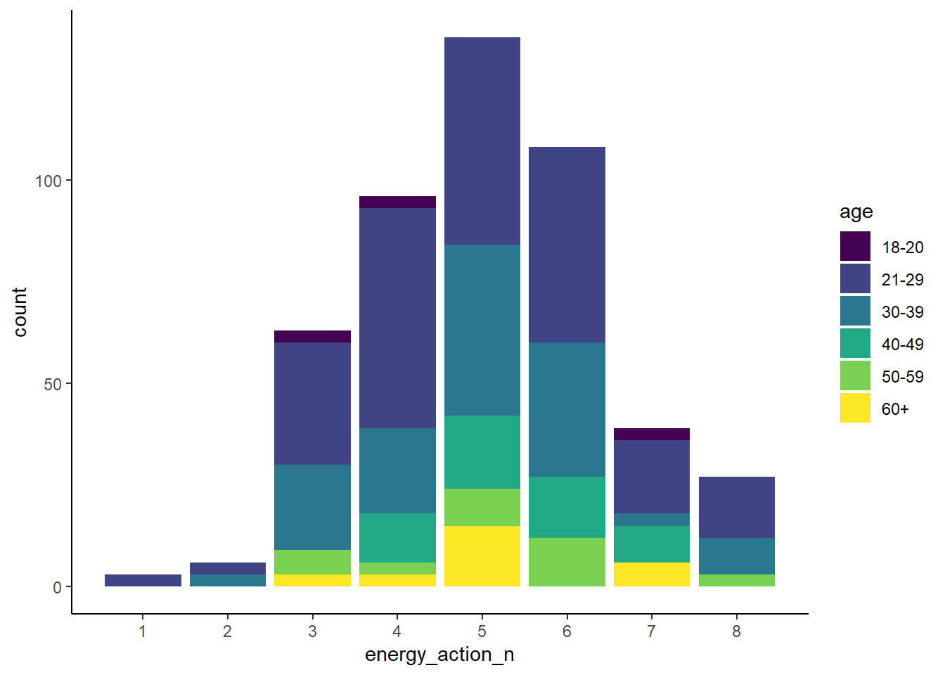
Basic stacked bar chart
To make a conventional stacked bar chart, we will use the question on “How many of these energy related sustainable actions do you perform?”, the responses to which are found in sust_data$energy_action. We will group the responses by age cohort.
First, we need to count the number of sustainable actions performed, like we did earlier:
sust_data$energy_action_n <- nchar(as.character(sust_data$energy_action))
Then create the plot. We will use a colourblind-friendly colour palette provided by the viridis package.
(barchart <- ggplot(sust_data, aes(x =energy_action_n, fill = age)) +
    geom_bar() +
    scale_fill_viridis_d() +
    scale_x_continuous(breaks = seq(1:8)) +
    theme_classic())
Note that putting your entire ggplot code in brackets () creates the graph and then shows it in the plot viewer. If you don’t have the brackets, you’ve only created the object, but haven’t visualized it. You would then have to call the object such that it will be displayed by just typing barplot after you’ve created the “barplot” object.
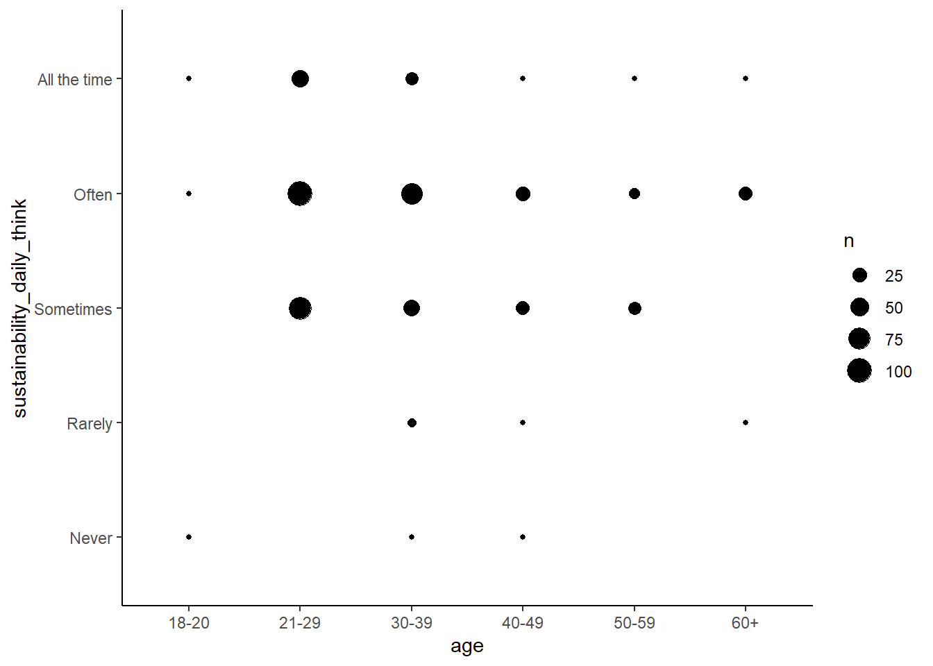
Bubble plot
If we want to compare correlations between two categories of data, we can use a bubble plot. For example, is there a pattern between age of respondent and how often they think about sustainable activities? The data from this survey doesn’t contain actual age values, only age ranges (e.g. 18-20, 21-29 etc.).
First, create a summary table by tallying the number of responses by the two groups, age and how often they think about sustainable activities:
sust_bubble <- sust_data %>%
	group_by(age, sustainability_daily_think) %>%
	tally()
Then to create the bubble plot, simply adjust the size of points according to their frequency of occurrence (n):
(bubbleplot <- ggplot(sust_bubble, aes(x = age, y = sustainability_daily_think)) +
	geom_point(aes(size = n)) +
	theme_classic())
3. Mining text responses and comments for keywords
As well as the tick box style questions, some questions in our survey asked for free-hand text comments. These comments give some extra information and context to survey responses and shouldn’t be ignored. As an example, look at first 20 elements of the column energy_action_comment by typing:
head(sust_data$energy_action_comment, 20)
We can mine the comments for keywords to build up a more complete picture of what our respondents were thinking about when they did the survey and whether that varies by gender. To make the comments easier to work with, we should make the data “tidy” by splitting each comment so that each row has a single word only.
Comments from all the questions
The following pipe collects all the comment columns along with the gender and id columns (dplyr::select()), then gathers those comment columns together into a single column (gather()), then transforms the comments column from a factor into a character class (mutate()). Note that we are using dplyr::select() instead of just select() - this is because often we have other packages loaded that might also have a select() function within them, so we want to explicitly state that we want to use the select() function from the dplyr package.
sust_comm_gather <- sust_data %>%
  dplyr::select(id, gender, energy_action_comment,
                food_action_comment, water_action_comment,
                waste_action_comment, other_action_comment) %>%
  gather(action, comment, -id, -gender) %>%
  mutate(comment = as.character(comment))
The next pipe takes that gathered data and uses unnest_tokens() from the tidytext package to split the comments so that there is only one word per row, then it uses the list of boring words from the stop_words object that we loaded earlier to remove those words from our dataset (filtering them out using filter() and the ! and %in% operators to remove words that occur in the stop_words$word column). We are also removing empty values !(is.na(comment_word)) and words that are actually just numbers (is.na(as.numeric(comment_word)). Then it counts the number of occurrences of each unique word in the comment_word column, by grouping by gender and summarising using the n() function. Finally a bit of tidying in the form of removing words which occur less than 10 times (filter(n > 10)).
sust_comm_tidy <- sust_comm_gather %>%
  unnest_tokens(output = comment_word,
                input = comment) %>%
  filter(!(is.na(comment_word)),
         is.na(as.numeric(comment_word)),
         !(comment_word %in% stop_words$word)) %>%
  group_by(gender, comment_word) %>%
  summarise(n = n()) %>%
  ungroup() %>%
  filter(n > 10)
Let’s define a custom colour palette for red and blue and name the colours after our gender categories:
male_female_pal <- c("#0389F0", "#E30031")
names(male_female_pal) <- c("Male", "Female")
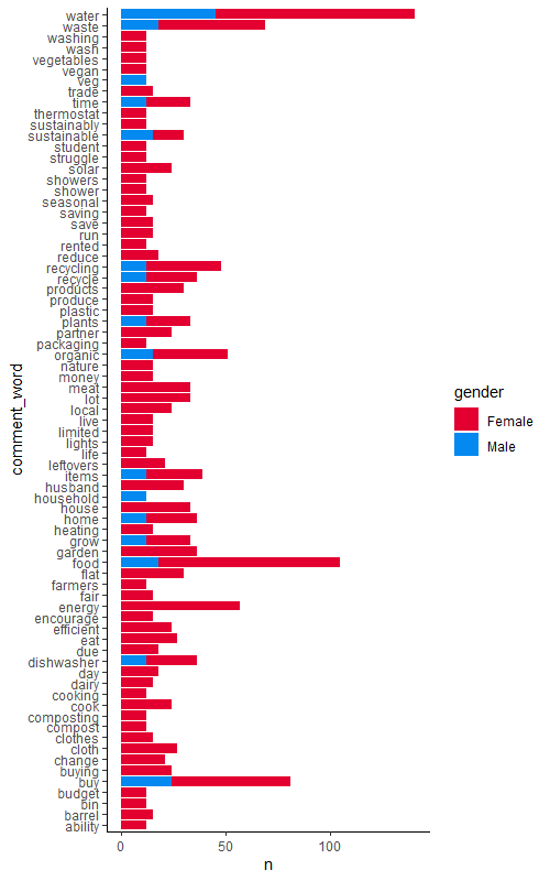
Now it is easy to plot the occurrences of each word, and colour by gender (fill = gender), using ggplot():
(occurrence <- ggplot(sust_comm_tidy, aes(x = comment_word, y = n, fill = gender)) +
	geom_bar(stat = "identity") +
	coord_flip() +
	scale_fill_manual(values = male_female_pal) +
	theme_classic())
Comments from a single question
We might also want to investigate a single question’s comments in more detail. For example, the energy_action_comment column. First repeat the action of converting to character format (mutate()), then filtering, summarising and grouping following a similar procedure as for the previous graph.
tidy_energy_often_comment <- sust_data %>%
  mutate(energy_action_comment = as.character(energy_action_comment)) %>%
  unnest_tokens(output = energy_action_comment_word,
                input = energy_action_comment) %>%
  filter(!(is.na(energy_action_comment_word)),
         is.na(as.numeric(energy_action_comment_word)),
         !(energy_action_comment_word %in% stop_words$word)) %>%
  group_by(gender, energy_action_comment_word) %>%
  summarise(n = n()) %>%
  ungroup()
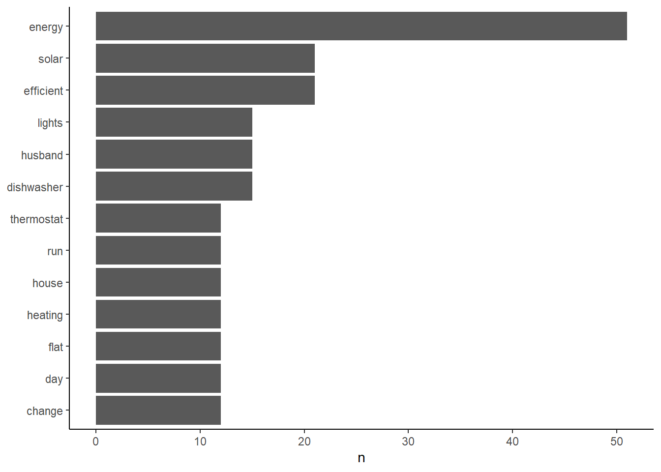
Then keep only the most common words and plot it as a bar chart:
tidy_energy_often_comment_summ <- tidy_energy_often_comment %>%
  filter(n > 10) %>%
  mutate(energy_action_comment_word = reorder(energy_action_comment_word, n ))

(most_common_plot <- ggplot(tidy_energy_often_comment_summ, aes(x = energy_action_comment_word, y = n)) +
    geom_col() +
    xlab(NULL) +  # this means we don't want an axis title
    coord_flip() +
    theme_classic())
Wordclouds
To effectively plot more words and their frequencies, you could also create a word cloud:
tidy_energy_often_comment %>%
	with(wordcloud(words = energy_action_comment_word, freq = n, max.words = 100))
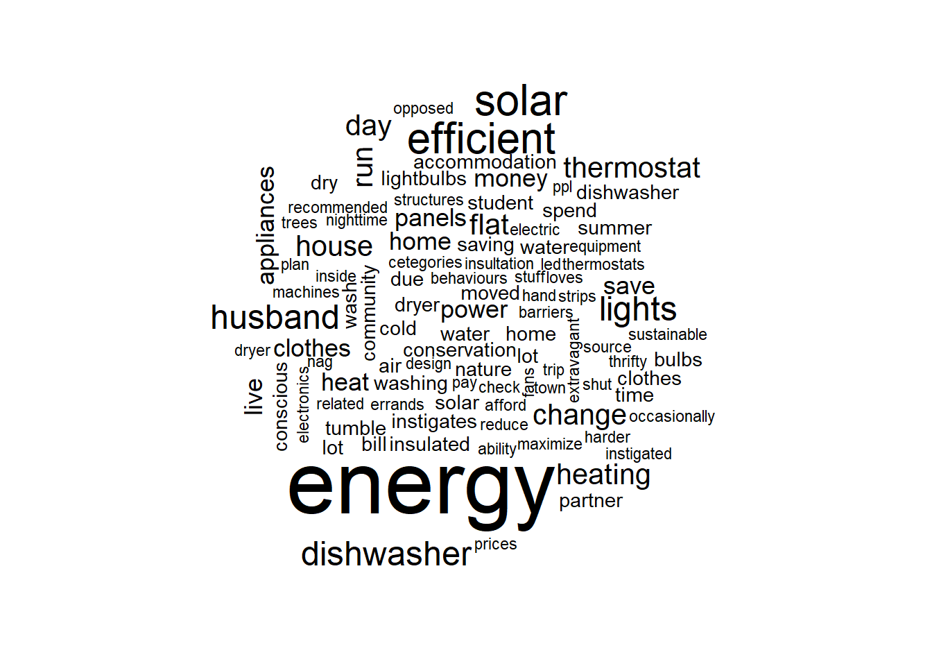
For more on text mining using tidytext, you can check out the Gitbook website.
4. Analyse qualitative data
Due to the way survey data are usually formatted, with lot of counts and factors, the assumptions of conventional parametric statistical analysis are often violated, so we can branch out from our usual linear models! Below are a few examples of how to test various hypotheses using our survey data.
Chi-squared
To test if there is a statistically significant correlation between gender and how often sustainable tasks are though about, we can use a chi-squared test of independence.
gender_think_chi <- chisq.test(sust_data$gender, sust_data$sustainability_daily_think)
gender_think_chi
The output of the gender_think_chi object can be used to interpret the outcome of the chi-squared test, with a lower p-value indicating a greater probability that the two variables are dependent on each other. In this case, p = 0.01572, which is lower than the conventional threshold of 0.05, meaning we can reject the null hypothesis that gender does not correlate with the frequency at which people think about sustainable tasks.
Poisson regression
For a more in depth analysis, we might hypothesise that gender causes the difference in the number of energy related sustainable actions performed. This is in contrast to the Chi-squared test which merely suggests a non-directional correlative tendency between the two variables. As the number of actions performed is count data, we can use a Poisson regression, which is a type of a generalised linear model:
energy_action_pois <- glm(energy_action_n ~ gender, family = "poisson", data = sust_data)
summary(energy_action_pois)
In this case it seems like there actually isn’t much effect of gender on number of actions performed, with a very low z-value of 0.457 and a non-significant p-value (0.648). This means we can accept the null hypothesis that gender does not affect the number of sustainable energy actions performed.
Multi-variate Poisson regression
Going deeper, we might hypothesise that gender and age interact to determine the amount of sustainable food related actions. For example, maybe the difference between genders becomes more accentuated as age increases. Including age in our model might help to make the model fit better and explain more variance. This effect can be included in a generalised linear model as an “interaction term”. In the code below gender * age defines the interaction between those two explanatory variables:
energy_action_pois_int <- glm(energy_action_n ~ gender * age, family = "poisson", data = sust_data)
summary(energy_action_pois_int)
We don’t find support for our hypothesis that gender differences increase with age, as the effect size for the interaction term is very small.
Conclusion
In this tutorial, we learned how to visualise qualitative data using different types of plots, as well as how to analyse the data to test different hypotheses, hopefully getting you one step closer to unwrapping your data presents!