Tutorial aims & steps:
- Customise histograms in
ggplot2 - Create your own colour palette
- Customise boxplots in
ggplot2 - Add regression lines to your plots
- Create your own ggplot theme
- Challenge yourself!
Following from our first tutorial on data visualisation using ggplot2, we are now back for more ggplot2 practice and customisation. Since no two figures are ever the same, the ability to customise your figures is key. The ultimate aim of this tutorial is to help you to make your figures even more beautiful and informative!
Downloading data
We will use made-up data consisting of the abundance and height of different plant species occurring in two magic lands: Hogsmeade and Narnia.
The imaginary data for this tutorial can be downloaded from this repository. Clone and download the repo as a zipfile, then unzip and set the folder as your working directory by running the code below (replacing with your actual folder path), or clicking Session/ Set Working Directory/ Choose Directory from the RStudio menu.
Alternatively, you can fork the repository to your own GitHub account and then add it as a new RStudio project by copying the HTTPS/SSH link. For more details on how to register on GitHub, download Git, sync RStudio and Github and use version control, please check out our Git tutorial.
Make a new script file through clicking File/ New File/ R Script, give it a title and some information, and we are all set to explore how plant communities have changed in our magical lands: Hogsmeade and Narnia!
## Vegetation of magical lands
## Data visualisation tutorial
## YOUR NAME
## DATE
#
# Load libraries ----
library(dplyr)  # For data manipulation
library(ggplot2)  # For data visualisation

setwd("PATH_TO_FOLDER")  # Set working directory to the folder where you saved the data

# Read in data ----
magic_veg <- read.csv("magic_veg.csv")
We will first explore our dataset using the str() function, which shows what type each variable is. What is the dataset made of?
str(magic_veg)

# land - the location within the land of magic (two possible lands: Narnia and Hogsmeade)
# plot - the plot number within each land
# year - the year the measurement was taken
# species - the species name (or code), Note that these are fake species!
# height - the imaginary canopy height at that point
# id - the id of each observation
1. Customise histograms in ggplot2
We’ll start by revisiting some of the types of plots we can make with ggplot2. Let us first calculate how many species there are in each plot.
species_counts <- magic_veg %>%
  group_by(land, plot) %>%
  summarise(Species_number = length(unique(species)))
Using what we’ve learnt from our previous data visualisation tutorial, we run the following code to create a histogram.
(hist <- ggplot(species_counts, aes(x = plot)) +
  geom_histogram())
Note that putting your entire ggplot code in brackets () creates the graph and then shows it in the plot viewer. If you don’t have the brackets, you’ve only created the object, but haven’t visualised it. You would then have to call the object such that it will be displayed by just typing hist after you’ve created the “hist” object.
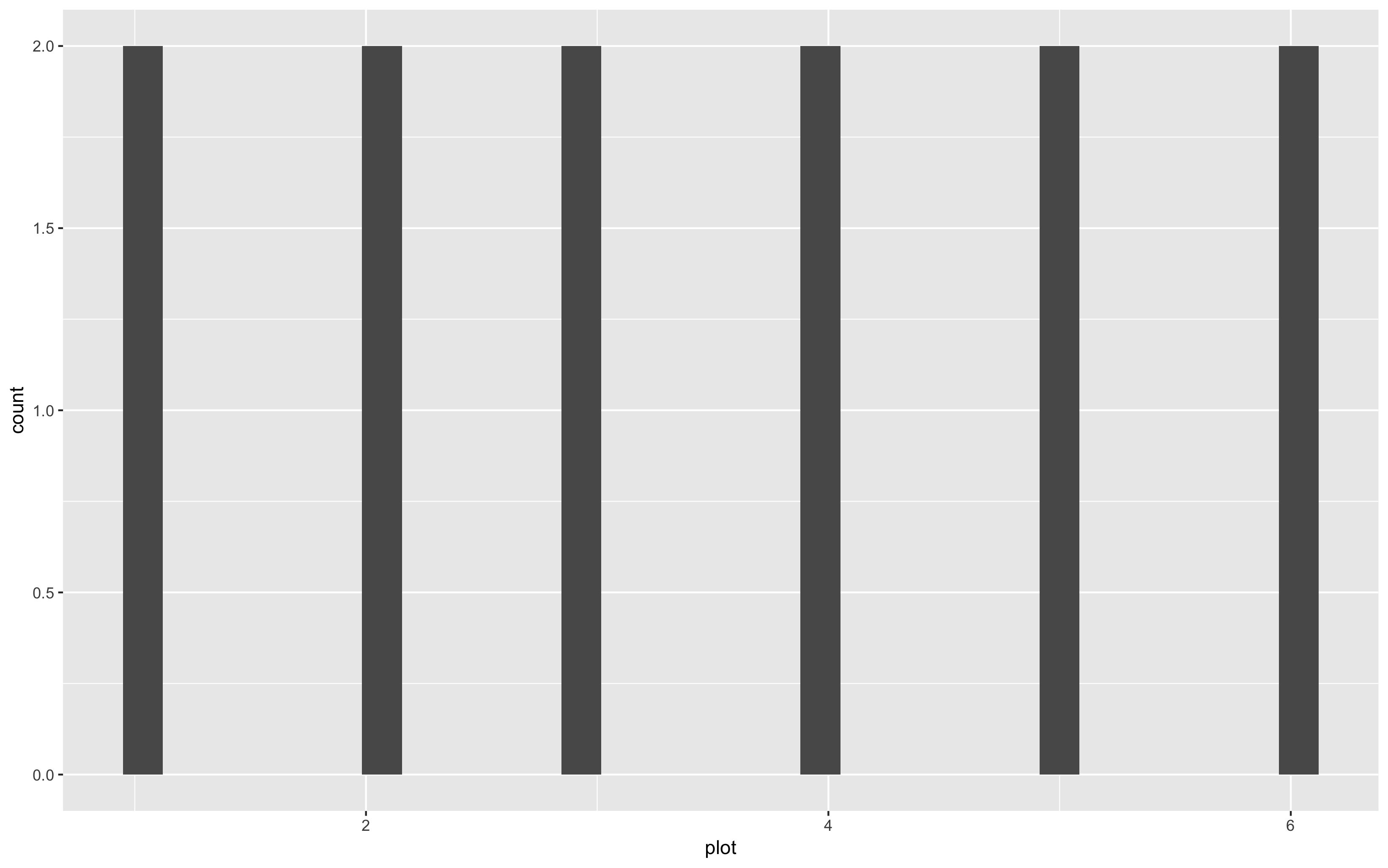 Uh, oh… That’s a weird histogram!
This is the common way of making a histogram, when you have one observation per row and the histogram tallies them for you. But you can immediately see that it doesn’t look right, because we are working with summarised data. You therefore need to tell R that you already know how many species are in each plot. You do that by specifying the stat argument:
(hist <- ggplot(species_counts, aes(x = plot, y = Species_number)) +
    geom_histogram(stat = "identity"))

# Note: an equivalent alternative is to use geom_col (for column), which takes a y value and displays it
(col <- ggplot(species_counts, aes(x = plot, y = Species_number)) +
   geom_col()
   )
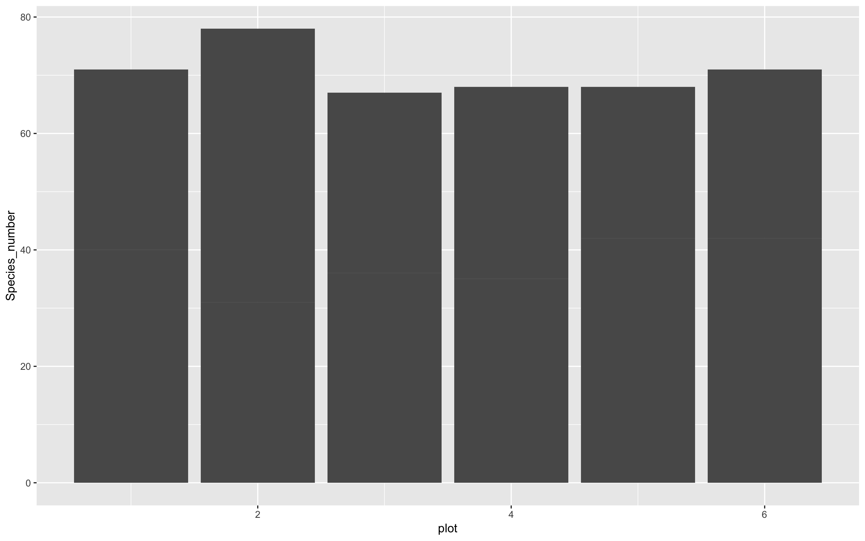
That looks a bit better, but it still seems to have far too many species. That’s because plots from each land are being grouped together. We can separate them by introducing a colour code, and make a stacked bar plot like this:
(hist <- ggplot(species_counts, aes(x = plot, y = Species_number, fill = land)) +
  geom_histogram(stat = "identity"))

# Remember that any aesthetics that are a function of your data (like fill here) need to be INSIDE the aes() brackets.
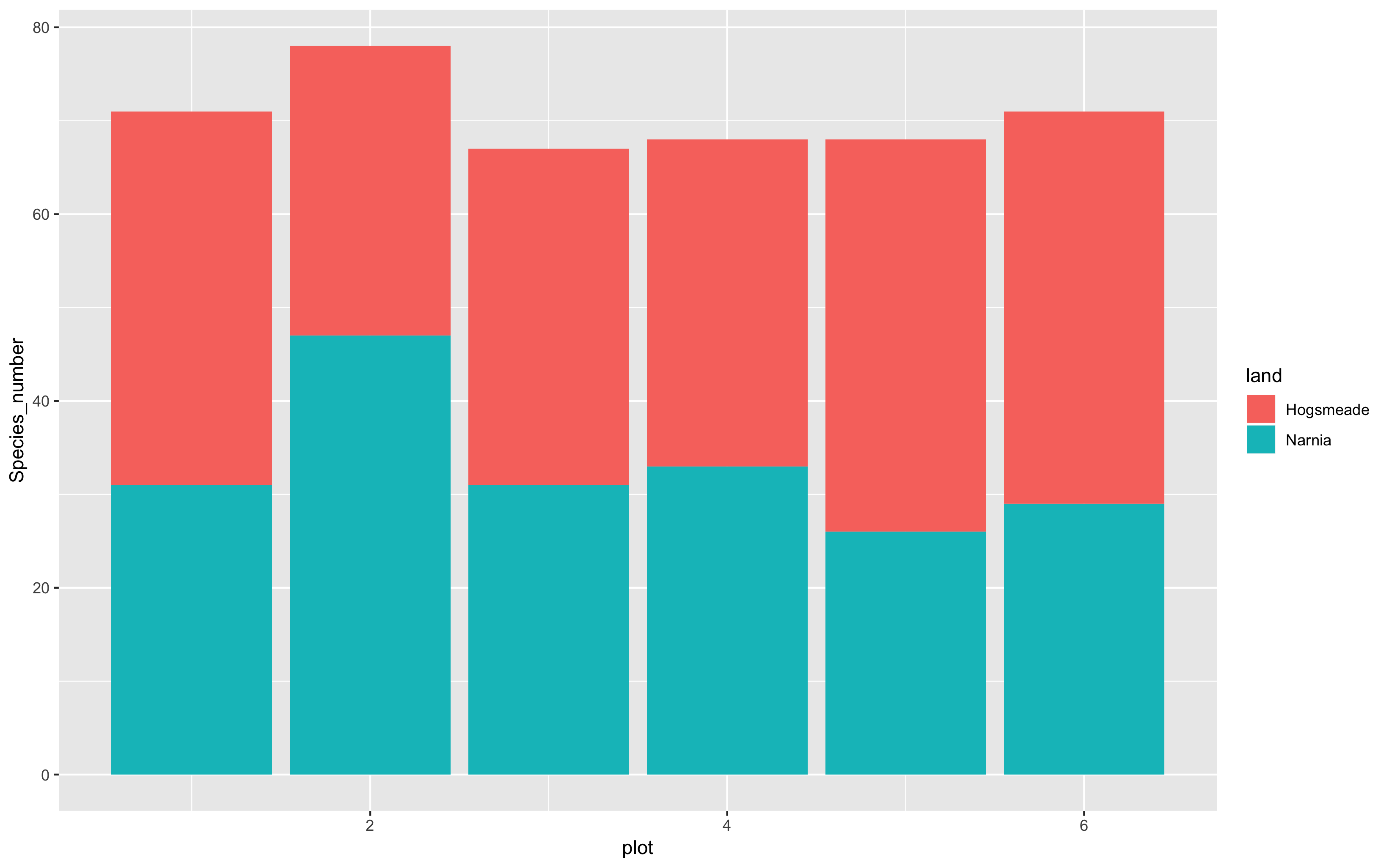
And if we want to make the columns to appear side by side rather than being stacked, you add position = "dodge" to the geom’s arguments.
(hist <- ggplot(species_counts, aes(x = plot, y = Species_number, fill = land)) +
    geom_histogram(stat = "identity", position = "dodge"))
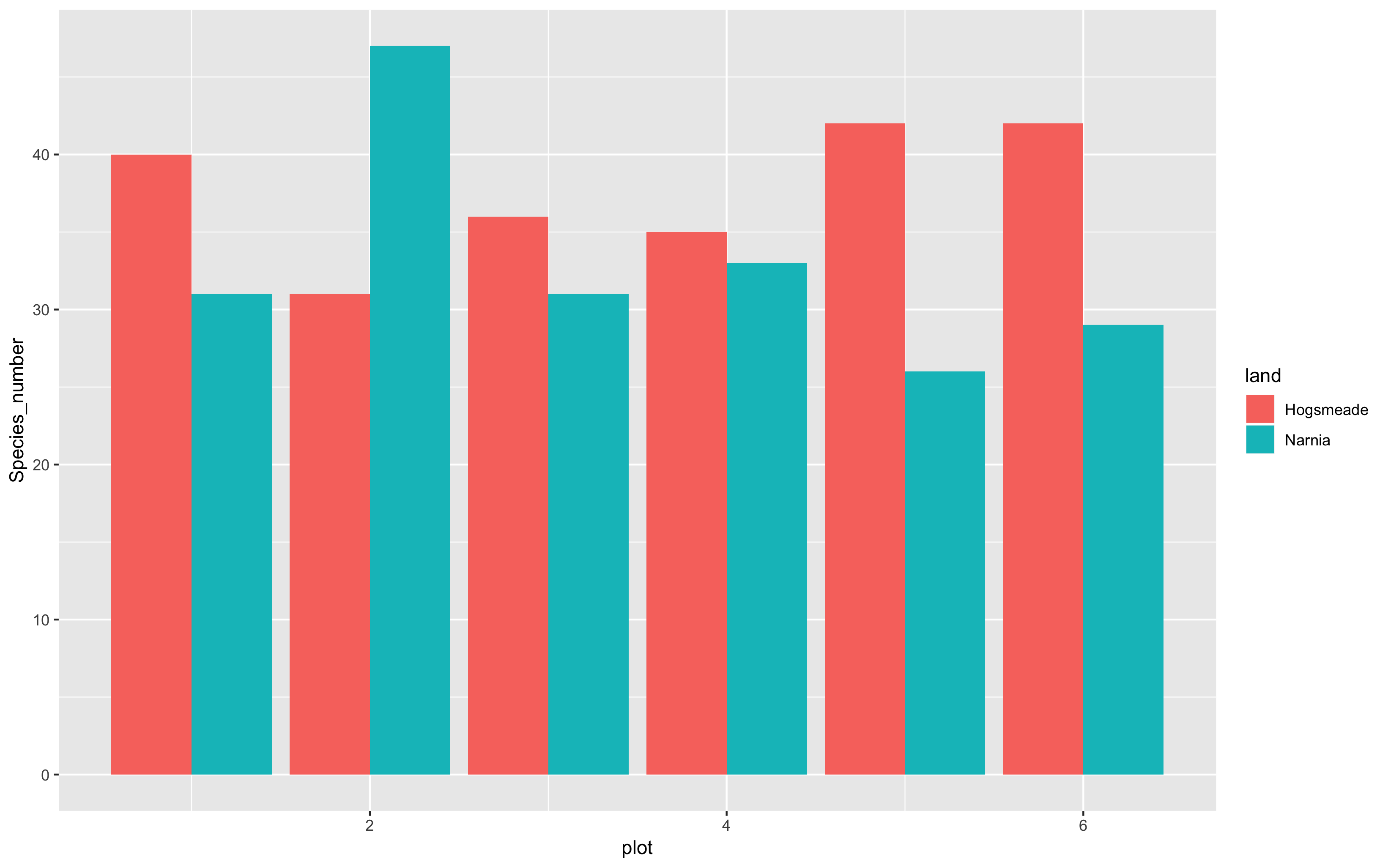 That’s certainly much better… not perfect though!
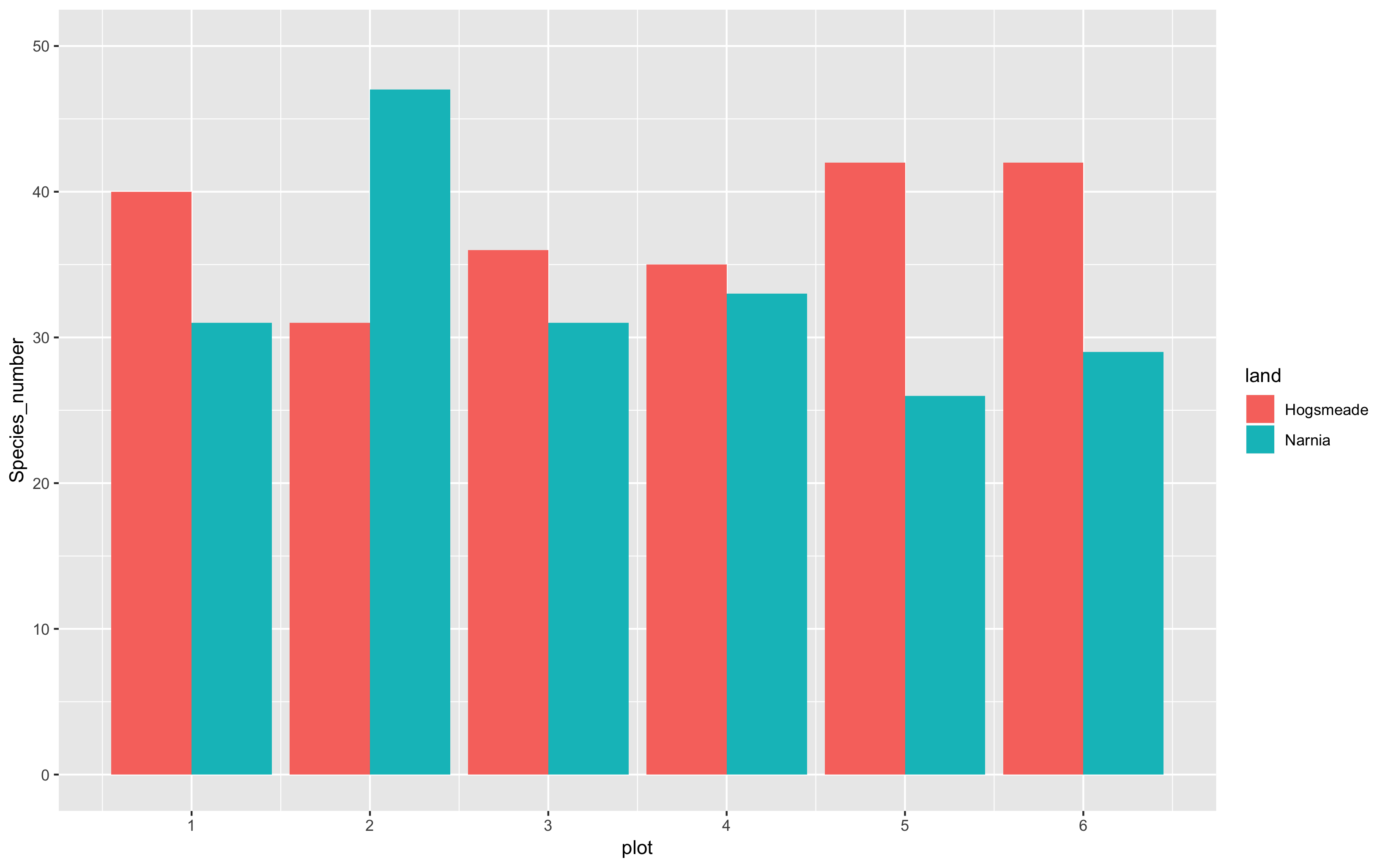
Note how our figure only shows plot numbers 2, 4, and 6. If you want the axis to display every plot number, 1 - 6, you can run the following code using breaks = c(1,2,3,4,5,6) or using breaks = 1:6. We can also specify the limits of the plot axes - running the code below, you’ll be able to see that the limit of the y axis now extends to the value of 50! This helps us keep all our data within the axis labels that we have, in terms of the visualisation!
(hist <- ggplot(species_counts, aes(x = plot, y = Species_number, fill = land)) +
    geom_histogram(stat = "identity", position = "dodge") +
    scale_x_continuous(breaks = c(1,2,3,4,5,6)) +
    scale_y_continuous(limits = c(0, 50)))
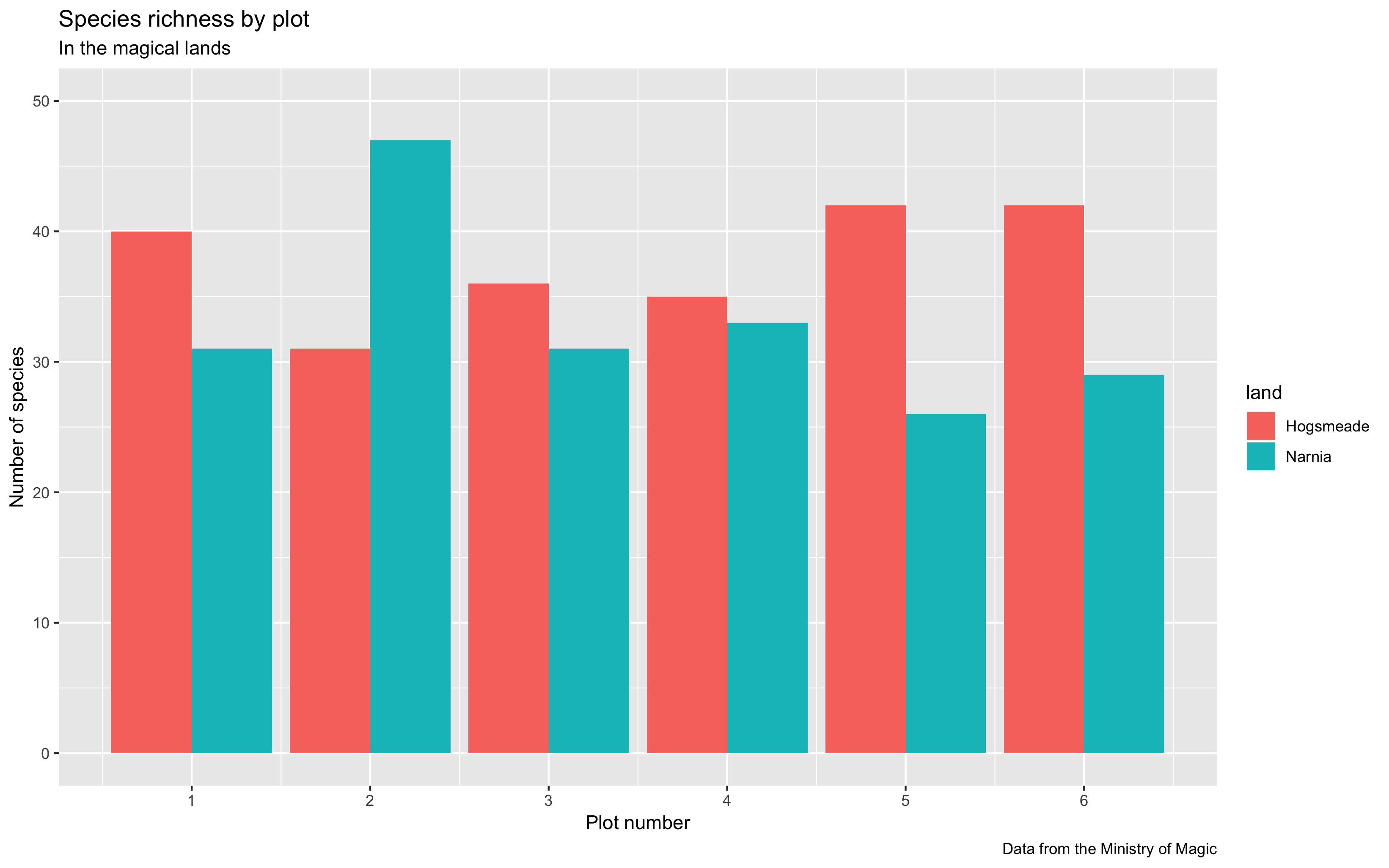
1a. Add titles, subtitles, captions and axis labels
Now it’s time for us to add more information to our graphs, for example, the plot title, subtitle, caption and axis labels. This might not be so useful in this case, but here’s some guidance just in case you do require this in your own work.
(hist <- ggplot(species_counts, aes(x = plot, y = Species_number, fill = land)) +
    geom_histogram(stat = "identity", position = "dodge") +
    scale_x_continuous(breaks = c(1,2,3,4,5,6)) +
    scale_y_continuous(limits = c(0, 50)) +
    labs(title = "Species richness by plot",
         subtitle = "In the magical lands",
         caption = "Data from the Ministry of Magic",
         x = "\n Plot number", y = "Number of species \n"))     # \n adds space before x and after y axis text
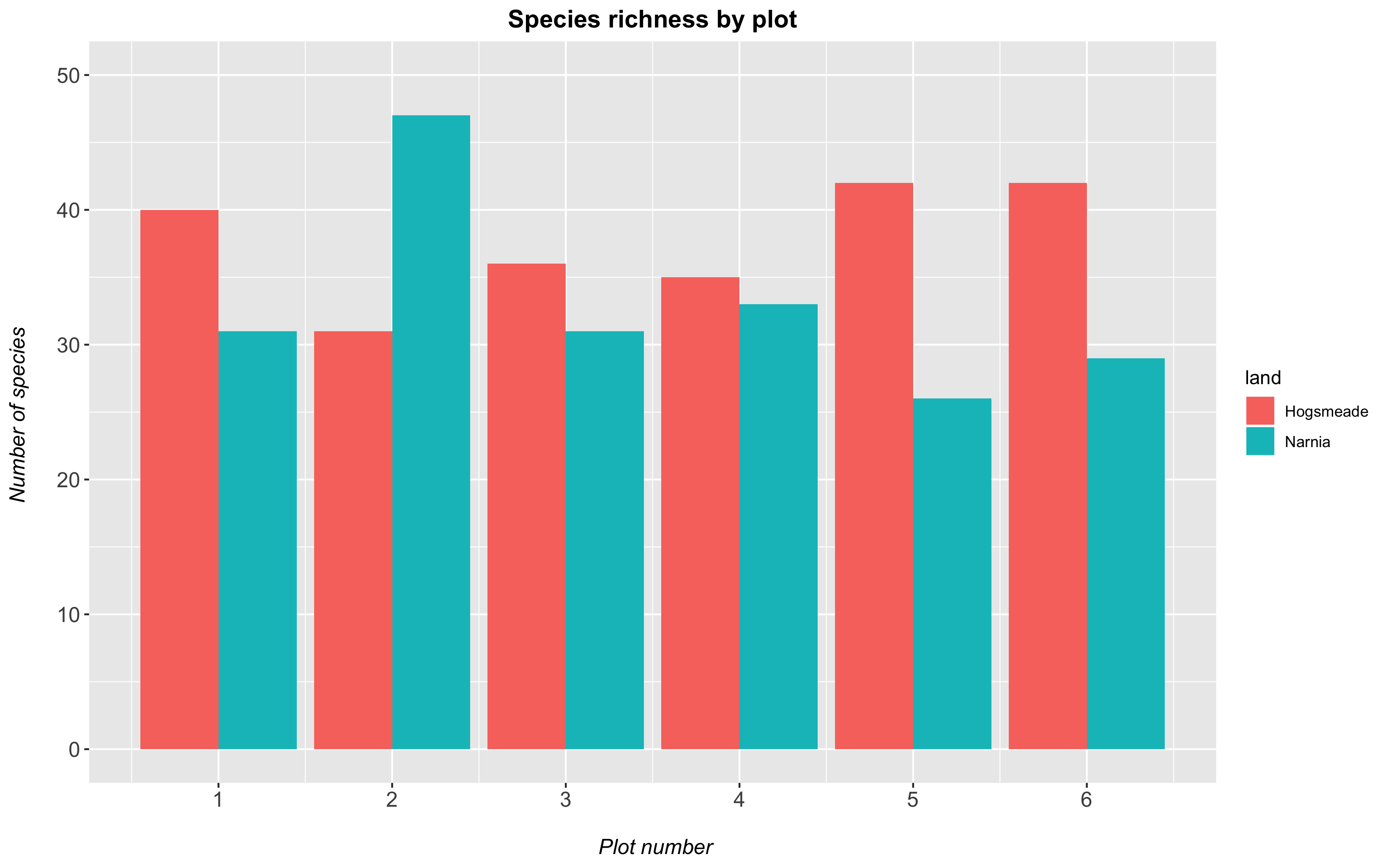
Control everything!
You can also add in theme() elements to your plot, which let you customise even more aspects! We already introduced theme elements in our previous tutorial. Here, we’re showing you how to change the font sizes of the axis label (axis text), axis title and plot title. Other things you can play around with are:
- italicise or bold the text with
face = 'italic'orface = 'bold'respectively - center the title using
hjust = 0.5
Note: if we wanted to specify different options for the x and y axis, we could use axis.text.x or axis.title.x and axis.text.y or axis.title.y and specify separate characteristics for each axis.
(hist <- ggplot(species_counts, aes(x = plot, y = Species_number, fill = land)) +
    geom_histogram(stat = "identity", position = "dodge") +
    scale_x_continuous(breaks = c(1,2,3,4,5,6)) +
    scale_y_continuous(limits = c(0, 50)) +
    labs(title = "Species richness by plot",
         x = "\n Plot number", y = "Number of species \n") +
    theme(axis.text = element_text(size = 12),
          axis.title = element_text(size = 12, face = "italic"),
          plot.title = element_text(size = 14, hjust = 0.5, face = "bold")))
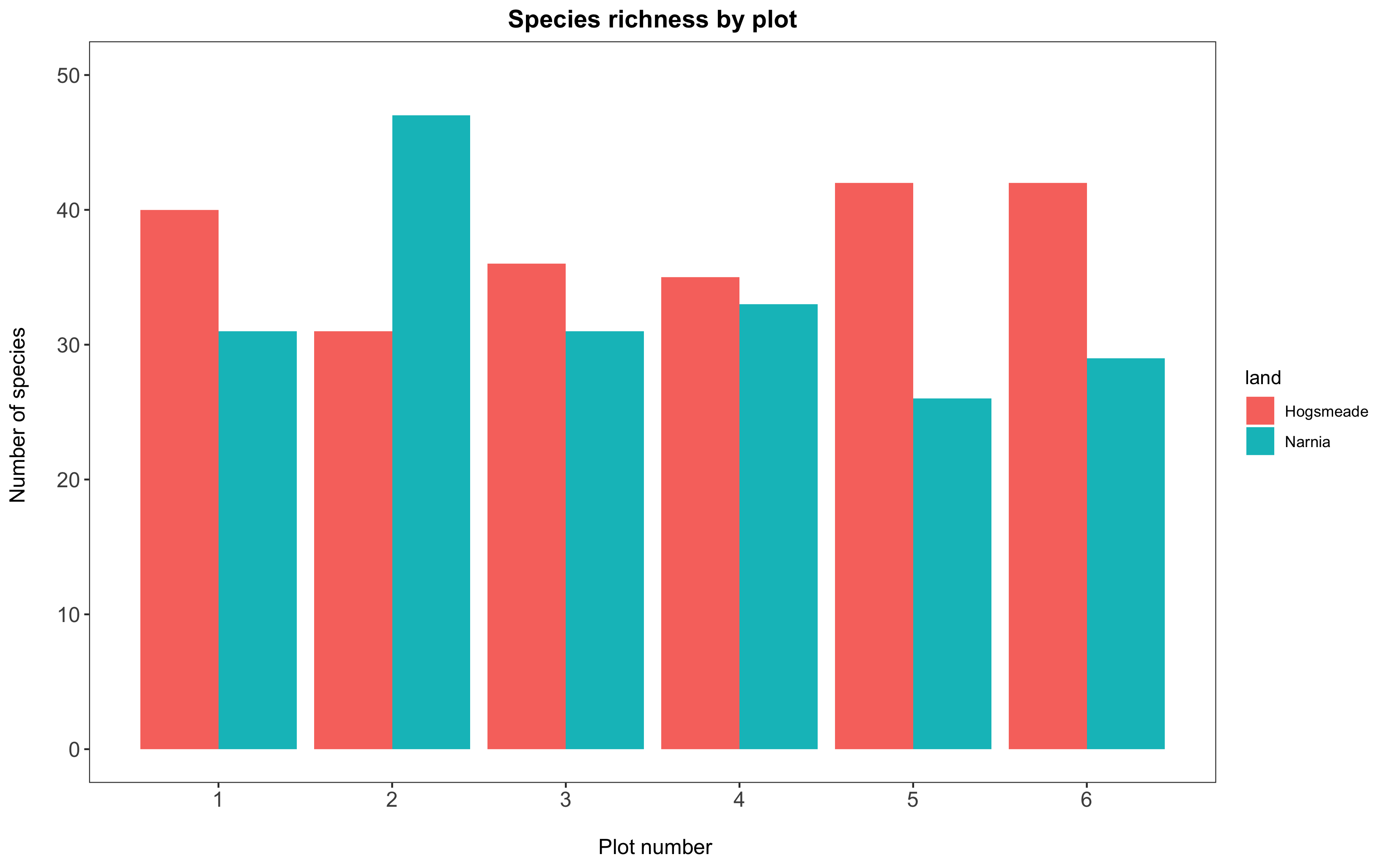
1b. Change the plot background
All our graphs at the moment still have a grey background, and honestly, we’re not a fan of it. It also has both major and minor grid lines for both the y and x axes, which we might want to remove to have a clear plain white background for the plot. Adding theme_bw() to our plot removes the grey background and replaces it with a white one. There are various other themes built into RStudio, but we personally think this is the cleanest one.
To remove the grid lines, we add the code panel.grid = element_blank() within the theme() command. Just like text.axis encompasses both text.axis.x and text.axis.y, panel.grid encompasses several options: panel.grid.major, which in turn governs panel.grid.major.x and panel.grid.major.y and the same for panel.grid.minor!
(hist <- ggplot(species_counts, aes(x = plot, y = Species_number, fill = land)) +
    geom_histogram(stat = "identity", position = "dodge") +
    scale_x_continuous(breaks = c(1,2,3,4,5,6)) +
    scale_y_continuous(limits = c(0, 50)) +
    labs(title = "Species richness by plot",
         x = "\n Plot number", y = "Number of species \n") +
    theme_bw() +
    theme(panel.grid = element_blank(),
          axis.text = element_text(size = 12),
          axis.title = element_text(size = 12),
          plot.title = element_text(size = 14, hjust = 0.5, face = "bold")))
1c. Fix the legend and customise the colours
We will use the scale_...() functions to customise both the color code AND the legend at once.
The scale_fill_manual(values = c("your-colour-1", "your-colour-2", ...)) function lets you decide on custom colour values for solid elements (bars, boxplots, ribbons, etc.), and its counterpart scale_colour_manual() works exactly the same for line elements (points in a scatter plot, regression lines, box or column outlines, etc.). You need to make sure you put in as many colours as there are factor levels in your data.
Need inspiration for your colours?
You can define colours using R’s built-in colour names or by specifying their Hex codes. The Colour Picker package is a great way to pick colours within the comfort of R Studio: see our previous tutorial for instructions on how to install it.
Also, notice how the name of our legend is now currently “land”: the title of that column in our dataframe species_counts. It is not very informative and not capitalized. We can change it to “Land of Magic,” by specifying name = "Land of Magic" in our function scale_fill_manual(). In some cases, we might not want to have a title for the legend at all, which you can do by specifying in scale_fill_manual, name = NULL.
(hist <- ggplot(species_counts, aes(x = plot, y = Species_number, fill = land)) +
    geom_histogram(stat = "identity", position = "dodge") +
    scale_x_continuous(breaks = c(1,2,3,4,5,6)) +
    scale_y_continuous(limits = c(0, 50)) +
    scale_fill_manual(values = c("rosybrown1", "#deebf7"),     # specifying the colours
                      name = "Land of Magic") +                # specifying title of legend
    labs(title = "Species richness by plot",
         x = "\n Plot number", y = "Number of species \n") +
    theme_bw() +
    theme(panel.grid = element_blank(),
          axis.text = element_text(size = 12),
          axis.title = element_text(size = 12),
          plot.title = element_text(size = 14, hjust = 0.5, face = "bold"),
          plot.margin = unit(c(0.5,0.5,0.5,0.5), units = , "cm"),
	  legend.title = element_text(face = "bold"),
          legend.position = "bottom",
          legend.box.background = element_rect(color = "grey", size = 0.3)))
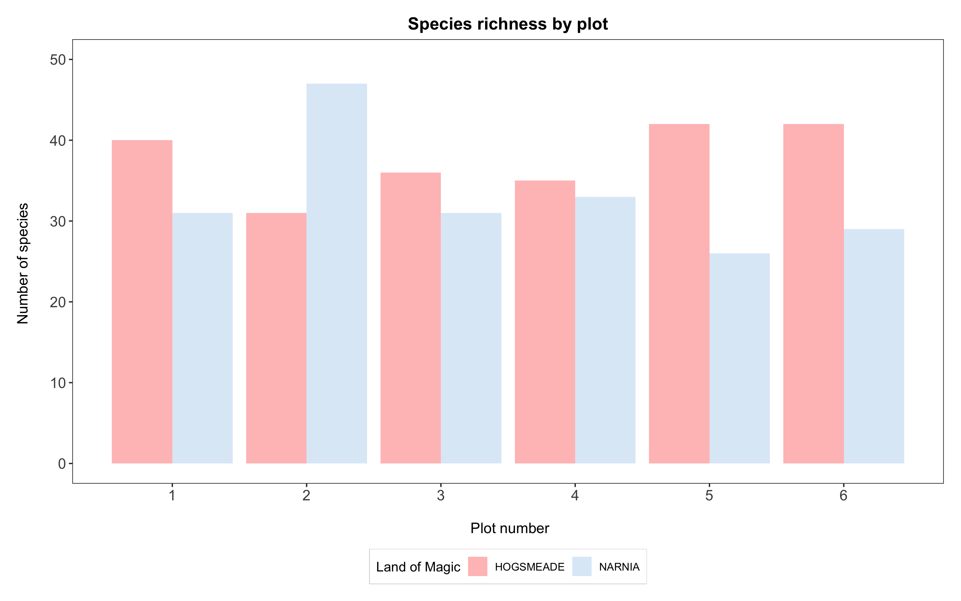
Another thing that we might sometimes want to change is the actual label of the group (i.e. the factor levels). In the following example, our dataframe has “Hogsmeade” and “Narnia” specified, which is lucky as they would reflect correctly in the legend built by ggplot. However, if it they had simply been listed as “group1” and “group2” in the original data file, we would want to have more informative labels. We can do that by manipulating labels = c("xxx", "xxx"). In the example below, we change the labels from the default (taking from the dataframe) of “Hogsmeade” and “Narnia” to “HOGSMEADE” and “NARNIA” just for demonstration purposes. Important: Make sure you list the new label names in the same order as your factors are listed in the dataset, otherwise you risk assigning the wrong group to the values! Use levels(dataframe$factorname)to see the factors in order (usually alphabetical).
(hist <- ggplot(species_counts, aes(x = plot, y = Species_number, fill = land)) +
    geom_histogram(stat = "identity", position = "dodge") +
    scale_x_continuous(breaks = c(1,2,3,4,5,6)) +
    scale_y_continuous(limits = c(0, 50)) +
    scale_fill_manual(values = c("rosybrown1", "#deebf7"),           # specifying the colours
                      labels = c("HOGSMEADE", "NARNIA"),             # changing the site labels
                      name = "Land of Magic") +                      # defining legend title
    labs(title = "Species richness by plot",
         x = "\n Plot number", y = "Number of species \n") +
    theme_bw() +
    theme(panel.grid = element_blank(),
          axis.text = element_text(size = 12),
          axis.title = element_text(size = 12),
          plot.title = element_text(size = 14, hjust = 0.5, face = "bold"),
          plot.margin = unit(c(0.5,0.5,0.5,0.5), units = , "cm"),
	  legend.title = element_text(face = "bold"),
          legend.position = "bottom",
          legend.box.background = element_rect(color = "grey", size = 0.3)))
Let’s cover some more of the theme() elements we’ve used in the examples above:
legend.titleallows you to change the font size of the legend, or its formatting (e.g. bold).- The
legend.positioncan be defined with accepted positions such as"bottom", but you can also dolegend.position = c(0.1, 0.8), which would bring the legend to the top left hand corner (corresponding to the x and y values on the graph). This is a neat trick in some cases, where you have lots of blank space within your plot itself and want to fine-tune the legend position. - Finally, we’ve used
legend.box.background = element_rect()to create a light grey rectangle that surrounds the legend. If you don’t want this, you can just remove that line of code.
To save a plot, we use the function ggsave() where you can specify the dimensions and resolution of your plot. You could also change the file ending with .png to .pdf to save your image as a PDF document. Note that this file will be saved into your working directory. (If you’ve forgotten where that is, you can find it by running the code getwd().)
Note: If you want your file to be saved in a specific folder that is within your working directory (for example, into an “images” folder), you can change the code from ggsave("magical-land-sp-richness.png") to ggsave("images/magical-land-sp-richness.png"). (Make sure you’ve created the folder first or you’ll run into an error!)
ggsave("magical-sp-rich-hist.png", width = 7, height = 5, dpi = 300)
 Congratulations, you’ve made a beautiful graph!
2. Create your own colour palette
When you have several factor levels and need to come up with a pretty, clear, and contrasting colour scheme, it is always a good idea to look online for inspiration. Some great websites we use are Colour Brewer or coolors. Colour Brewer even allows you to specify colourblind-safe palettes, which you definitely should want!
A more advanced use of colour palettes is to create one linked to your factor levels. This is great when you work on a project that will have multiple figures, and you want the colour-coding to be consistent across the board. Linking colours specifically to factor levels ensures that if a factor is dropped from a data frame, the corresponding colour will be dropped from the resulting plot, too, instead of being reassigned to the next available factor level.
Here with only two magical lands, you could easily keep track of the colours, but imagine if you had 10 different lands! Let’s create a fake dataframe of values for more magical lands, and see the power of this approach.
# Create vectors with land names and species counts
land <- factor(c("Narnia", "Hogsmeade", "Westeros", "The Shire", "Mordor", "Forbidden Forest", "Oz"))
counts <- as.numeric(c(55, 48, 37, 62, 11, 39, 51))

# Create the new data frame from the vectors
more_magic <- data.frame(land, counts)

# We'll need as many colours as there are factor levels
length(levels(more_magic$land))    # that's 7 levels

# CREATE THE COLOUR PALETTE
magic.palette <- c("#698B69", "#5D478B", "#5C5C5C", "#CD6090", "#EEC900", "#5F9EA0", "#6CA6CD")    # defining 7 colours
names(magic.palette) <- levels(more_magic$land)                                                    # linking factor names to the colours

# Bar plot with all the factors

(hist <- ggplot(more_magic, aes(x = land, y = counts, fill = land)) +
      geom_histogram(stat = "identity", position = "dodge") +
      scale_y_continuous(limits = c(0, 65)) +
      scale_fill_manual(values = magic.palette,                        # using our palette here
                        name = "Land of Magic") +
      labs(title = "Species richness in magical lands",
           x = "", y = "Number of species \n") +
      theme_bw() +
      theme(panel.grid = element_blank(),
            axis.text = element_text(size = 12),
            axis.text.x = element_text(angle = 45, hjust = 1),
            axis.title = element_text(size = 12),
            plot.title = element_text(size = 14, hjust = 0.5, face = "bold"),
            plot.margin = unit(c(0.5,0.5,0.5,0.5), units = , "cm"),
            legend.title = element_text(face = "bold"),
            legend.position = "bottom",
            legend.box.background = element_rect(color = "grey", size = 0.3)))


# See how consistent the colour scheme is if you drop some factors (using filter in the first line)

(hist <- ggplot(filter(more_magic, land %in% c("Hogsmeade", "Oz", "The Shire")), aes(x = land, y = counts, fill = land)) +
      geom_histogram(stat = "identity", position = "dodge") +
      scale_y_continuous(limits = c(0, 65)) +
      scale_fill_manual(values = magic.palette,                       # using our palette ensures that colours with no corresponding factors are dropped
                        name = "Land of Magic") +
      labs(title = "Species richness in magical lands",
           x = "", y = "Number of species \n") +
      theme_bw() +
      theme(panel.grid = element_blank(),
            axis.text = element_text(size = 12),
            axis.text.x = element_text(angle = 45, hjust = 1),
            axis.title = element_text(size = 12),
            plot.title = element_text(size = 14, hjust = 0.5, face = "bold"),
            plot.margin = unit(c(0.5,0.5,0.5,0.5), units = , "cm"),
            legend.title = element_text(face = "bold"),
            legend.position = "bottom",
            legend.box.background = element_rect(color = "grey", size = 0.3)))
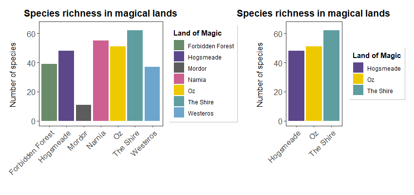 Notice the consistent colour coding when dropping factors!
Shades and gradients
So far we’ve used scale_colour_manual() and scale_fill_manual() to define custom colours for factor levels. But what if your variable is continuous rather than categorical, so that you can’t possibly assign a colour to every value? You might then want the colour scheme to go from light to dark according to the values, and scale_colour_gradient() (and its friend scale_fill_gradient()) are there for you (and might be useful for the challenge too, cough cough).
You can learn more about these functions here; basically, you just have to set your low = and high = colour values and the function will do the rest for you. We love it!
3. Customise boxplots in ggplot2
We could also plot the data using boxplots. Boxplots sometimes look better than bar plots, as they make more efficient use of space than bars and can reflect uncertainty in nice ways.
To make the boxplots, we will slightly reshape the dataset to take account of year as well. For more information on data manipulation using dplyr and pipes %>%, you can check out our data manipulation tutorial.
yearly_counts <- magic_veg %>%
  group_by(land, plot, year) %>%                             # We've added in year here
  summarise(Species_number = length(unique(species))) %>%
  ungroup() %>%
  mutate(plot = as.factor(plot))
We first can plot the basic boxplot, without all the extra beautification we’ve just learnt about to look at the trends.
(boxplot <- ggplot(yearly_counts, aes(plot, Species_number, fill = land)) +
  geom_boxplot())
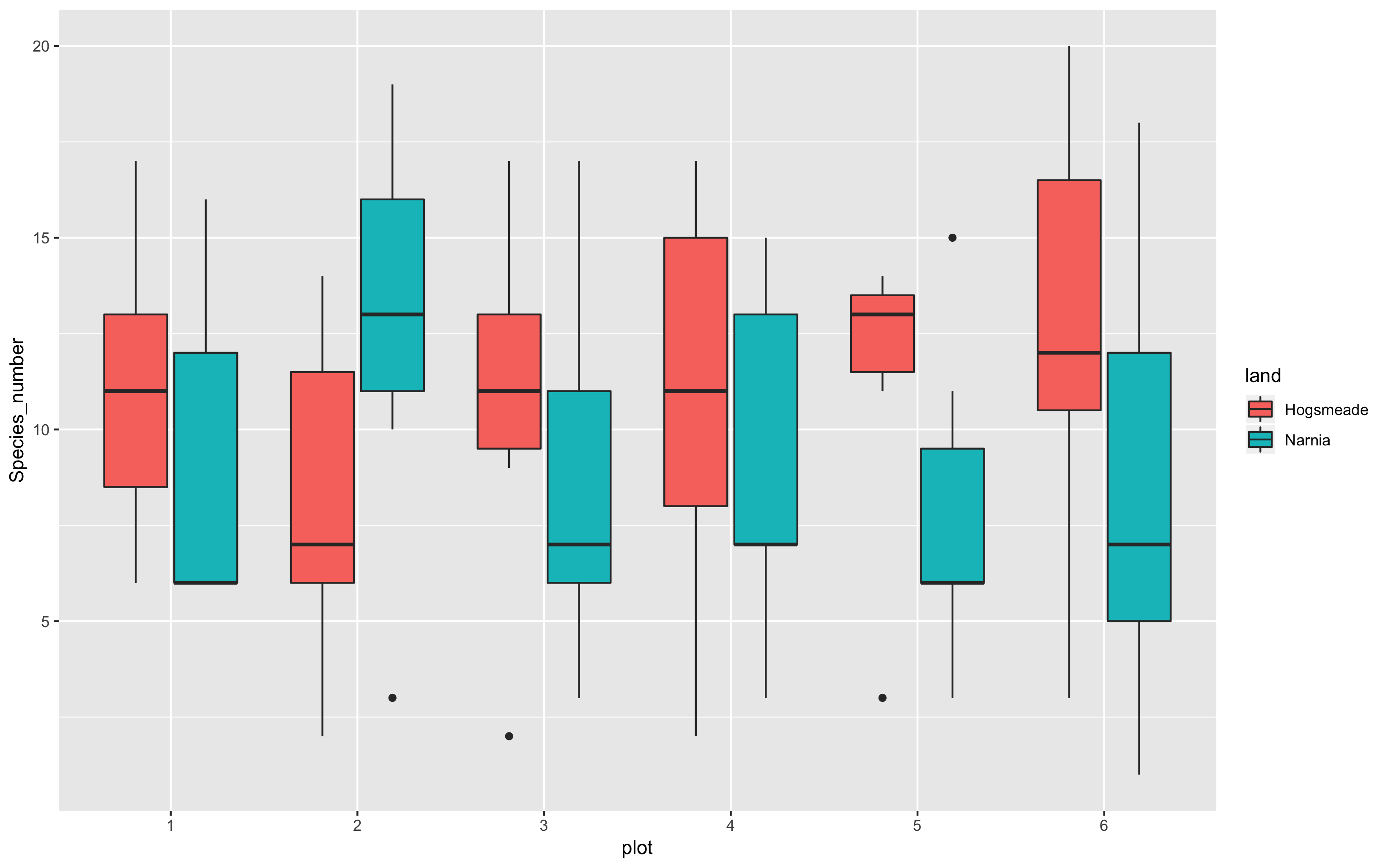
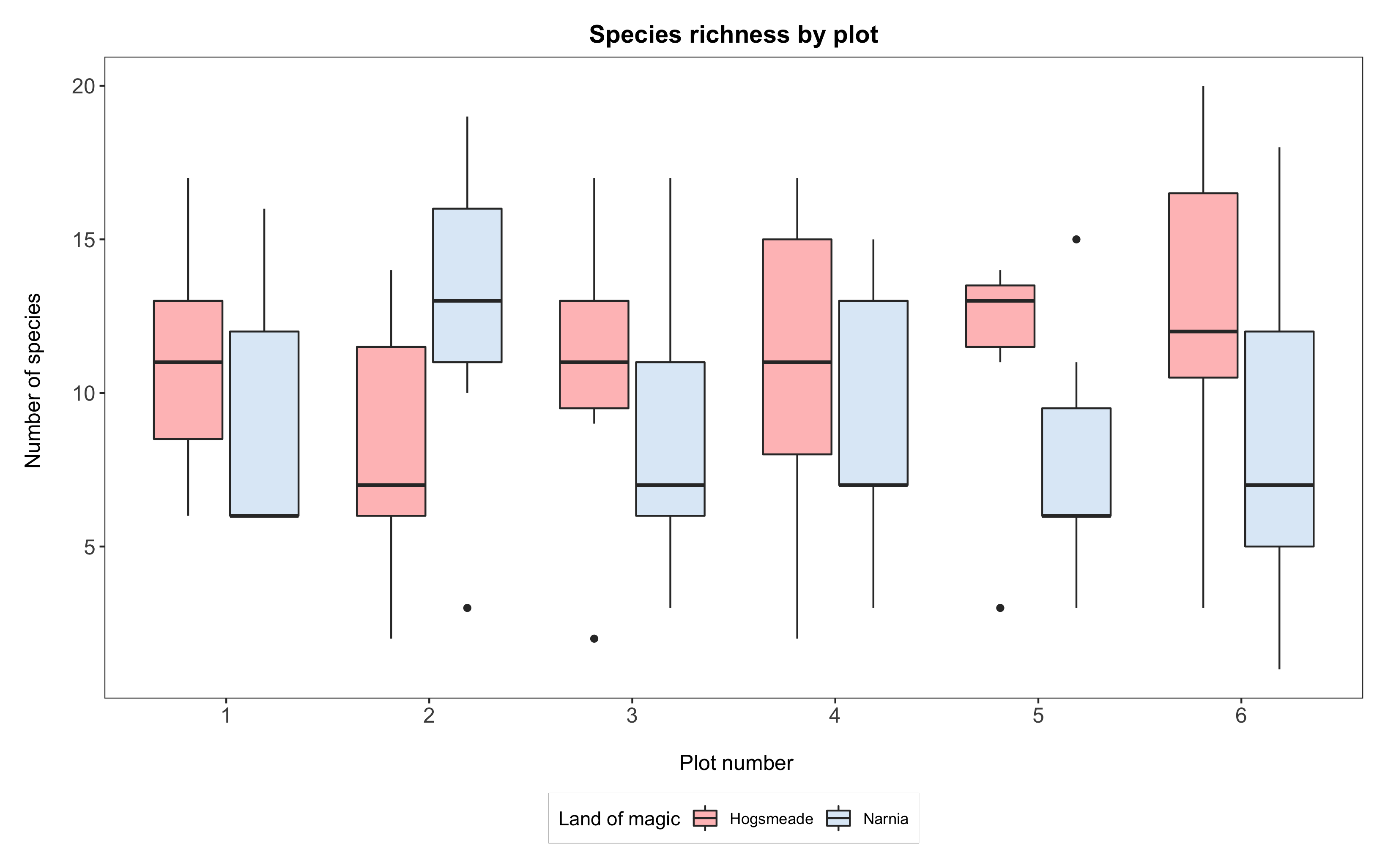
This does a much nicer job of showing which plots are the most species rich. With the beautifying customisations we’ve just learnt, we can make the plot much prettier!
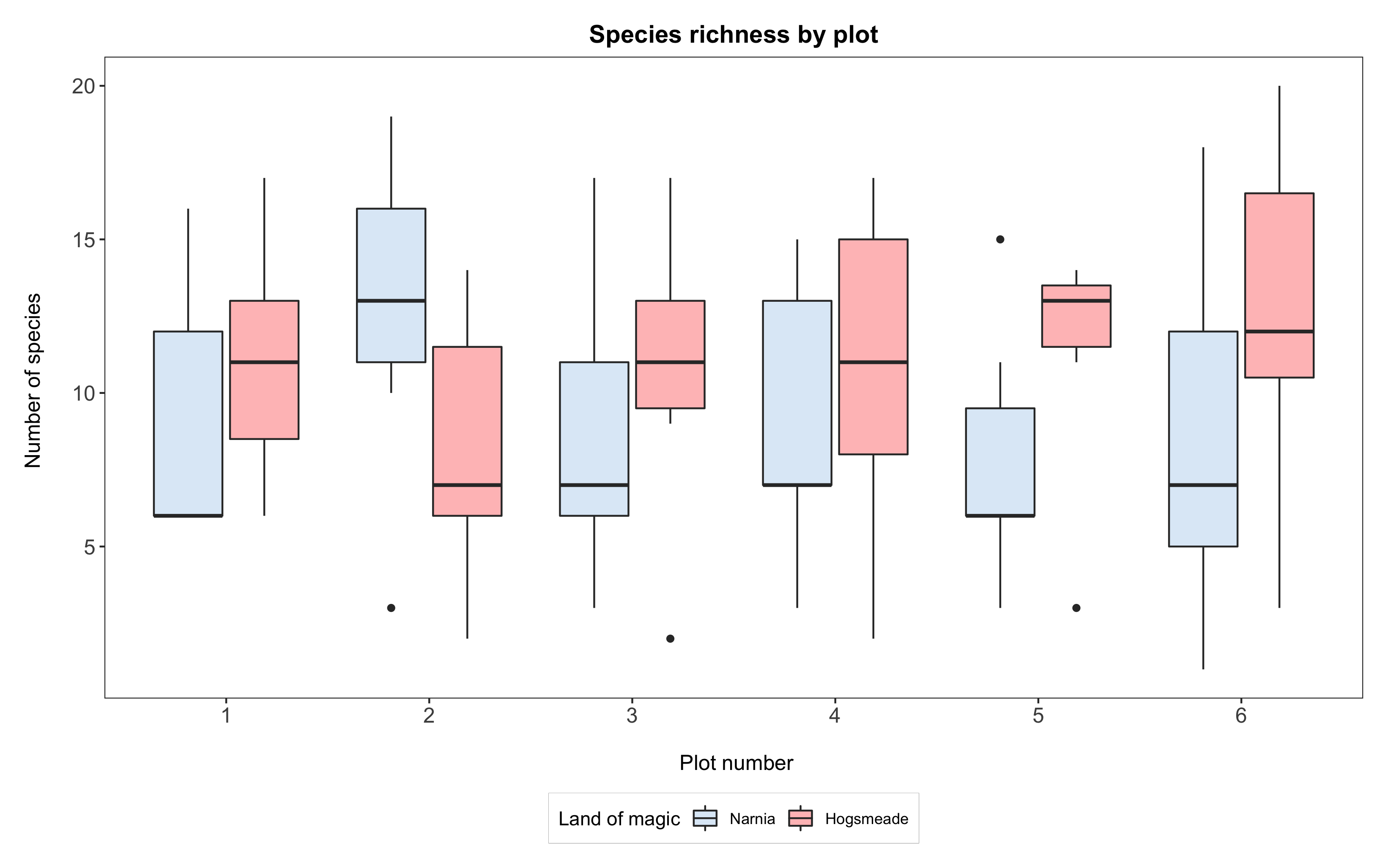
(boxplot <- ggplot(yearly_counts, aes(x = plot, y = Species_number, fill = land)) +
  geom_boxplot() +
  scale_x_discrete(breaks = 1:6) +
  scale_fill_manual(values = c("rosybrown1", "#deebf7"),
                    breaks = c("Hogsmeade","Narnia"),
                    name="Land of magic",
                    labels=c("Hogsmeade", "Narnia")) +
  labs(title = "Species richness by plot",
       x = "\n Plot number", y = "Number of species \n") +
  theme_bw() +
  theme() +
  theme(panel.grid = element_blank(),
        axis.text = element_text(size = 12),
        axis.title = element_text(size = 12),
        plot.title = element_text(size = 14, hjust = 0.5, face = "bold"),
        plot.margin = unit(c(0.5,0.5,0.5,0.5), units = , "cm"),
        legend.position = "bottom",
        legend.box.background = element_rect(color = "grey", size = 0.3)))

# Saving the boxplot
ggsave("magical-sp-rich-boxplot1.png", width = 7, height = 5, dpi = 300)
Box, bar, dot…?
Bar plots are very commonly used to show differences or ranking among groups. A problem with them, especially if used without a measure of uncertainty (e.g. error bars), is that what they display is a range of values starting from 0. If the variable you are plotting can reasonably have values of zero, then that’s fine, but often it’s improbable. For instance, we wouldn’t imagine that our lands of magic could be completely devoid of any life form and therefore have a species richness of zero. Same holds true if you’re comparing body weight, plant height, and a great majority of ecological variables!
An easy alternative is a dot plot, which you could have done by summarising the species_counts data to get a mean and standard deviation of species counts for each land. You’d then use geom_point(aes(x = land, y = mean)) rather than geom_histogram(), and add your uncertainty with geom_errorbar(aes(x = land, ymin = mean - sd, ymax = mean + sd).
# Create the summarised data
summary <- species_counts %>%  group_by(land) %>% summarise(mean = mean(Species_number),
                                                            sd = sd(Species_number))

# Make a dot plot
(dot <- ggplot(summary, aes(x = land, y = mean, colour = land)) +
      geom_errorbar(aes(ymin = mean - sd, ymax = mean + sd), width = 0.2) +
      geom_point(size = 3) +
      scale_y_continuous(limits = c(0, 50)) +
      scale_colour_manual(values = c('#CD5C5C', '#6CA6CD'),
                        labels = c('HOGSMEADE', 'NARNIA'),
                        name = 'Land of Magic') +
      labs(title = 'Average species richness',
           x = '', y = 'Number of species \n') +
      theme_bw() +
      theme(panel.grid = element_blank(),
            axis.text = element_text(size = 12),
            axis.title = element_text(size = 12),
            plot.title = element_text(size = 14, hjust = 0.5, face = 'bold'),
            plot.margin = unit(c(0.5,0.5,0.5,0.5), units = , 'cm'),
            legend.title = element_text(face = 'bold'),
            legend.position = 'bottom',
            legend.box.background = element_rect(color = 'grey', size = 0.3)))
Boxplots, just like dot plots, give a more accurate idea of the range of values in your data: but remember that the thicker line in the box represents the median, not the mean!
Reordering factors
Remember how we learnt to recode and reorder factors in our advanced data manipulation tutorial? We often want to do this so that we can plot values in a specific order.
If we wanted to have Narnia come before Hogsmeade, we would first have to reorder the data in the dataframe. From this point, after reordering the data, ggplot will always plot Narnia before Hogsmeade. Also, note how we’ve changed the order of things in scale_fill_manual - above we had it as “Hogsmeade”, then “Narnia”, and now we have “Narnia” come before “Hogsmeade” to also reorder the legend.
# Reordering the data
yearly_counts$land <- factor(yearly_counts$land,
                             levels = c("Narnia", "Hogsmeade"),
                             labels = c("Narnia", "Hogsmeade"))

# Plotting the boxplot
(boxplot <- ggplot(yearly_counts, aes(x = plot, y = Species_number, fill = land)) +
    geom_boxplot() +
    scale_x_discrete(breaks = 1:6) +
    scale_fill_manual(values = c("#deebf7", "rosybrown1"),
                      breaks = c("Narnia","Hogsmeade"),
                      name = "Land of magic",
                      labels = c("Narnia", "Hogsmeade")) +
    labs(title = "Species richness by plot",
         x = "\n Plot number", y = "Number of species \n") +
    theme_bw() +
    theme() +
    theme(panel.grid = element_blank(),
          axis.text = element_text(size = 12),
          axis.title = element_text(size = 12),
          plot.title = element_text(size = 14, hjust = 0.5, face = "bold"),
          plot.margin = unit(c(0.5,0.5,0.5,0.5), units = , "cm"),
          legend.position = "bottom",
          legend.box.background = element_rect(color = "grey", size = 0.3)))
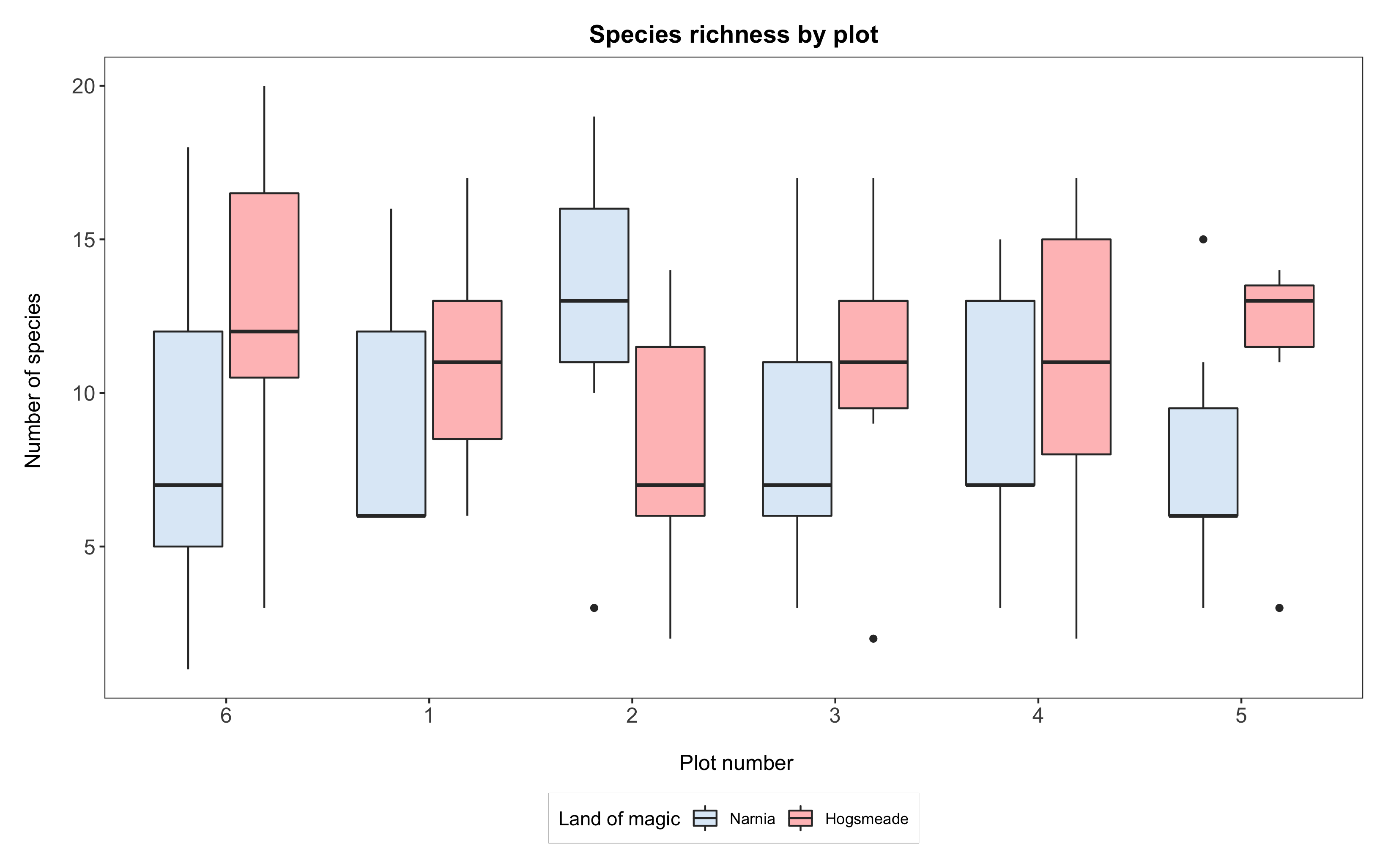
If we wanted to reorder the y axis of plot numbers, such that the boxplot for plot 6 comes before 1, then 2, 3, 4, 5, we can use the same principle. Again, from this point on, ggplot will always plot “6” before the rest.
# Reordering the data
yearly_counts$plot <- factor(yearly_counts$plot,
                             levels = c("6", "1", "2", "3", "4", "5"),
                             labels = c("6", "1", "2", "3", "4", "5"))

# Plotting the boxplot
(boxplot2 <- ggplot(yearly_counts, aes(x = plot, y = Species_number, fill = land)) +
    geom_boxplot() +
    scale_x_discrete(breaks = 1:6) +
    scale_fill_manual(values = c("#deebf7", "rosybrown1"),
                      breaks = c("Narnia","Hogsmeade"),
                      name = "Land of magic",
                      labels = c("Narnia", "Hogsmeade")) +
    labs(title = "Species richness by plot",
         x = "\n Plot number", y = "Number of species \n") +
    theme_bw() +
    theme() +
    theme(panel.grid = element_blank(),
          axis.text = element_text(size = 12),
          axis.title = element_text(size = 12),
          plot.title = element_text(size = 14, hjust = 0.5, face = "bold"),
          plot.margin = unit(c(0.5,0.5,0.5,0.5), units = , "cm"),
          legend.position = "bottom",
          legend.box.background = element_rect(color = "grey", size = 0.3)))
4. Plot regression lines onto your plots
We are now going to look at another aspect of the data: the plant heights, and how they might have changed over time. First, we need to do a little bit of data manipulation to extract just the heights:
heights <- magic_veg %>%
  filter(!is.na(height)) %>%                    # removing NA values
  group_by(year, land, plot, id) %>%
  summarise(Max_Height = max(height)) %>%       # Calculating max height
  ungroup() %>%                                 # Need to ungroup so that the pipe doesn't get confused
  group_by(year, land, plot) %>%
  summarise(Height = mean(Max_Height))          # Calculating mean max height
We can view this as a basic scatterplot in ggplot2:
(basic_mm_scatter <- ggplot(heights, aes(year, Height, colour = land)) +
  geom_point() +
  theme_bw())
We can see pretty clear trends over time, and so we can try to plot a simple straight line through this using stat_smooth in ggplot2, by specifying a linear model (lm) method. We did this briefly at the end of our first ggplot tutorial.
(basic_mm_scatter_line <- ggplot(heights, aes(year, Height, colour = land)) +
  geom_point() +
  theme_bw() +
  stat_smooth(method = "lm"))
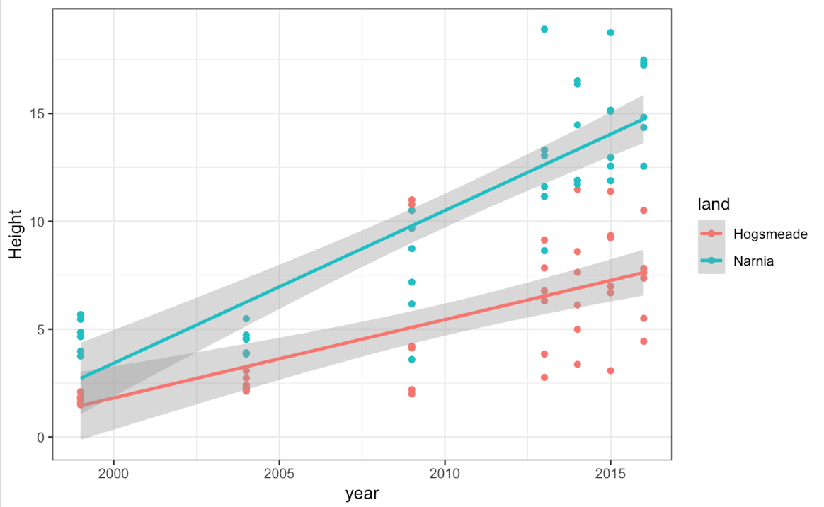
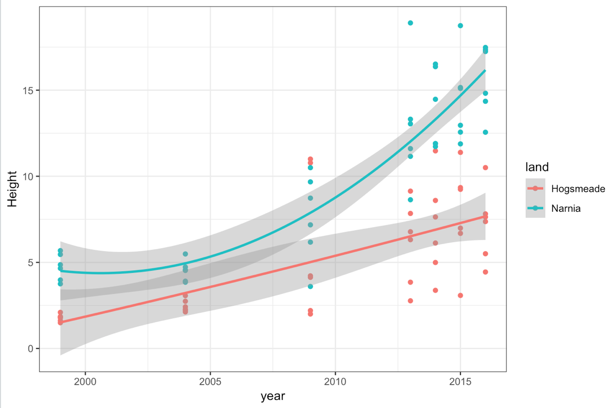
However, perhaps this isn’t what we really want, because you can see the relationship isn’t linear. An alternative would be to use a different smoothing equation. Let’s try a quadratic fit - something slightly more complicated to produce than the standard fits provided by R. Thankfully, ggplot2 lets us customise to pretty much any type of fit we want, as we can add in an equation to tell it what to plot. There are also several different base fits available. You can check out some here.
(improved_mm_scat <- ggplot(heights, aes(year, Height, colour = land)) +
  geom_point() +
  theme_bw() +
  stat_smooth(method = "lm", formula = y ~ x + I(x^2)))
What about fancier stats?
Some of you might have picked up on the fact that our data are nested (species within plots within magic lands) and come from different years: therefore, a mixed-effects modelling approach might be better here. For an introduction to linear mixed effects modelling, check out our tutorial, where we show how to plot the model predictions.
For now, take some time to explore the different ggplot2 fits! For instance, method = "loess" gives a smoothed curve.
5. Creating your own ggplot theme
You might have noticed that the lines starting with theme() quickly pile up. We’ve been adjusting the font size of the axes and the labels, the position of the title, the background colour of the plot, etc. And then we’ve been copying and pasting those many lines of codes on all of our graphs, which really increases the length of our script, and makes our code less readable.
Here is a simple solution: create a customised theme that combines all the theme() elements you want! You can then apply it to your graphs to make things easier and increase consistency. You can include as many elements in your theme as you want, and when you apply your theme to a graph, only the relevant elements will be considered - e.g. for our histograms we won’t need to use legend.position, but it’s fine to keep it in the theme in case any future graphs we apply it to do have the need for legends.
theme_coding <- function(){            # creating a new theme function
  theme_bw()+                          # using a predefined theme as a base
  theme(axis.text.x = element_text(size = 12, angle = 45, vjust = 1, hjust = 1),       # customising lots of things
        axis.text.y = element_text(size = 12),
        axis.title = element_text(size = 14),
        panel.grid = element_blank(),
        plot.margin = unit(c(0.5, 0.5, 0.5, 0.5), units = , "cm"),
        plot.title = element_text(size = 20, vjust = 1, hjust = 0.5),
        legend.text = element_text(size = 12, face = "italic"),
        legend.title = element_blank(),
        legend.position = c(0.9, 0.9))
}
You can try out the effects of the theme by replacing all the code starting with theme(........) with just theme_coding(). Look at examples 1 and 2: they do the same thing, but #2 is so much easier to read!
# EXAMPLE 1: boxplot with all the theme elements specified

(boxplot <- ggplot(yearly_counts, aes(x = plot, y = Species_number, fill = land)) +
      geom_boxplot() +
      scale_x_discrete(breaks = 1:6) +
      scale_fill_manual(values = c("#deebf7", "rosybrown1"),
                        breaks = c("Narnia","Hogsmeade"),
                        name = "Land of magic",
                        labels = c("Narnia", "Hogsmeade")) +
      labs(title = "Species richness by plot",
           x = "\n Plot number", y = "Number of species \n") +
      theme_bw()+                          # using a predefined theme as a base
      theme(axis.text.x = element_text(size = 12, angle = 45, vjust = 1, hjust = 1),       # customising lots of things
            axis.text.y = element_text(size = 12),
            axis.title = element_text(size = 14),
            panel.grid = element_blank(),
            plot.margin = unit(c(0.5, 0.5, 0.5, 0.5), units = , "cm"),
            plot.title = element_text(size = 20, vjust = 1, hjust = 0.5),
            legend.text = element_text(size = 12, face = "italic"),
            legend.title = element_blank(),
            legend.position = c(0.9, 0.9))
)

# EXAMPLE 2: Using our custom theme to achieve the exact same thing

(boxplot <- ggplot(yearly_counts, aes(x = plot, y = Species_number, fill = land)) +
      geom_boxplot() +
      scale_x_discrete(breaks = 1:6) +
      scale_fill_manual(values = c("#deebf7", "rosybrown1"),
                        breaks = c("Narnia","Hogsmeade"),
                        name = "Land of magic",
                        labels = c("Narnia", "Hogsmeade")) +
      labs(title = "Species richness by plot",
           x = "\n Plot number", y = "Number of species \n") +
      theme_coding()                      # short and sweeeeet!
)


# And if you need to change some elements (like the legend that encroaches on the graph here), you can simply overwrite:

(boxplot <- ggplot(yearly_counts, aes(x = plot, y = Species_number, fill = land)) +
      geom_boxplot() +
      scale_x_discrete(breaks = 1:6) +
      scale_fill_manual(values = c("#deebf7", "rosybrown1"),
                        breaks = c("Narnia","Hogsmeade"),
                        name = "Land of magic",
                        labels = c("Narnia", "Hogsmeade")) +
      labs(title = "Species richness by plot",
           x = "\n Plot number", y = "Number of species \n") +
      theme_coding() +                      # this contains legend.position = c(0.9, 0.9)
      theme(legend.position = "right")      # this overwrites the previous legend position setting
)
6. Challenge yourself!
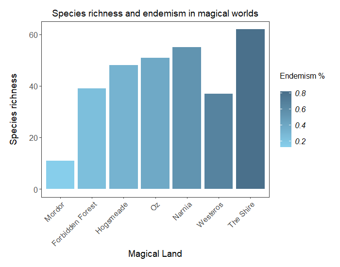
If you are keen for more practice, try this challenge! We’ll give you percentage of species that are endemic for our extended range of magical lands, and you will have to plot the species richness as a bar plot, coloured not by land this time, but with a shade representing the % of endemism. ( Hint: we mention this in one of our info boxes.)
You will need to append the endemism values to the more_magic data frame:
# Add % of endemic species to the data frame
more_magic <- more_magic %>% mutate(endemic = c(0.54, 0.32, 0.66, 0.80, 0.14, 0.24, 0.39))
And you’re all set to go! For an additional challenge, try ordering the bars so that they range from lowest to highest percentage of endemism. ( Hint: you might want to check the help on the reorder() function - it can even be used on the fly in the ggplot code!)
Click this line to view a solution
# Creating the bar plot

(endemic <- ggplot(more_magic, aes(x = land, y = counts, fill = endemic)) +   # colour coding by % endemic species
   geom_histogram(stat = 'identity') +
   scale_fill_gradient(low = '#87CEEB', high = '#4A708B',                     # creating gradient from pale to dark blue
                       name = 'Endemism % \n') +                              # setting legend title
   labs(x = 'Magical Land', y = 'Species richness \n',
   title = 'Species richness and endemism in magical worlds') +               # setting axes and main titles
   theme_coding() +
   theme(legend.position = 'right',                     # changing the legend position
         legend.title = element_text(size = 12),        # adding the legend title back
         plot.title = element_text(size = 14))           # reducing size of main title
)

# Reordering factor levels of land by % endemism (directly within aes() with reorder function)

(endemic <- ggplot(more_magic, aes(x = reorder(land, endemic), y = counts, fill = endemic)) +
      geom_histogram(stat = 'identity') +
      scale_fill_gradient(low = '#87CEEB', high = '#4A708B',                     # creating gradient from pale to dark blue
                          name = 'Endemism % \n') +                              # setting legend title
      labs(x = 'Magical Land', y = 'Species richness \n',
      title = 'Species richness and endemism in magical worlds') +               # setting axes and main titles
      theme_coding() +
      theme(legend.position = 'right',                     # changing the legend position
            legend.title = element_text(size = 12),        # adding the legend title back
            plot.title = element_text(size = 14))           # reducing size of main title
)

Doing this tutorial as part of our Data Science for Ecologists and Environmental Scientists online course?
This tutorial is part of the Stats from Scratch stream from our online course. Go to the stream page to find out about the other tutorials part of this stream!
If you have already signed up for our course and you are ready to take the quiz, go to our quiz centre. Note that you need to sign up first before you can take the quiz. If you haven't heard about the course before and want to learn more about it, check out the course page.