Advanced data manipulation

Created by Jakub Wieczorkowski

Tutorial Aims:

1. Appreciate the variety of functions in dplyr package and understand the potential for further learning.
2. Learn to creatively combine tables.
3. Become efficient and creative in manipulating variables and cases.

Tutorial Steps:

1. Introduction

Part I: Ocean animals

2. Combining tables:

a) combining rows with bind_rows

b) comparing data with set operations

c) combining tables with mutating joins

d) combining tables with filtering joins

e) challenge

Part II: Oceania LPI data

3. Manipulating variables:

a) extracting variables: select() and others

b) renaming variables: rename() and others

c) making new variables: mutate() and others

4. Manipulating cases:

a) extracting cases: filter() and others

b) adding cases: add_row()

5. Extra: Green Sea Turtle population trend

1. Introduction

You might have some experience in the basics of data manipulation and you know what pipes (%>%) are, but you are eager to learn some new variations of the functions you already know AND learn new ones? Then this tutorial is definitely for you!

The idea behind it is to make some more advanced aspects of data manipulation clearer, and to take a moment to learn a few new functions. The package dplyr (one of the packages from tidyverse) is your best friend for solving various challenges that you can encounter doing data manipulation.

We’ll go through dplyr functions together to make you more aware of their diversity. You will also become more efficient with the functions you already know by making small changes in the code, these will be e.g. my favourite functions select() and mutate(). You will probably spend an hour or so going through the tutorial - this will depend on how well you already know dplyr! However, in the long term, you will save yourself time from having to read through the endless information on the internet on why you keep getting errors or simply not getting the answer you want with the dplyr functions you thought you already knew (which has been my struggle for some time!). We’ll also cover a few other functions from other tidyverse packages to improve your confidence in data manipulation skills.

In PART I, we’ll be working with a fictional ocean animals dataset - to make the learning of combining tables less scary than it would be with large data frames. Then, in PART II, we’ll dive into the manipulation of variables and cases based on Living Planet dataset on marine organisms in Oceania. So, before you put on your scuba diving equipment for PART II, grab your snorkelling mask and we’re ready to start!

Part I: Ocean Animals

Create a new, blank script in RStudio and add tutorial title, your name, and the date at the top. When going through the tutorial, copy the individual code chunks and paste them to your script. Use # when adding comments.

Set the working directory, add the libraries, and load the multiple datasets.

# Title: Creative Data Manipulation: familiarising with the diversity of dplyr
# Your name
# Date

# Set working directory to where you saved the folder with tutorial materials on your computer
setwd("file-path")

# Libraries ----
library(dplyr)
# when we add new libraries throughout the tutorial, you can paste them here

# If you've never used a given package, install it with `install.packages("name")`

# Most of them are a part of `tidyverse` but we will be loading them separately so that you are aware of the contexts in which they are used

### PART I: OCEAN ANIMALS ----

# Load the datasets
animal_p1 <- read.csv("data/animal_p1.csv")
animal_p2 <- read.csv("data/animal_p2.csv")
animal_rp <- read.csv("data/animal_rp.csv")
animal_meal <- read.csv("data/animal_meal.csv")

To give you some background on PART I: imagine you have collected this data with your research partner when visiting a coral reef at Palmyra Atoll, a small island in the middle of the Pacific (fig. 1). You successfully managed to identify 10 animals of four different types (going down to the species level was not expected because you don’t necessarily need to be a marine biologist to do this tutorial!). Our aim is to combine different data tables, which we’ll then use to display average weight and meal type for each animal type!

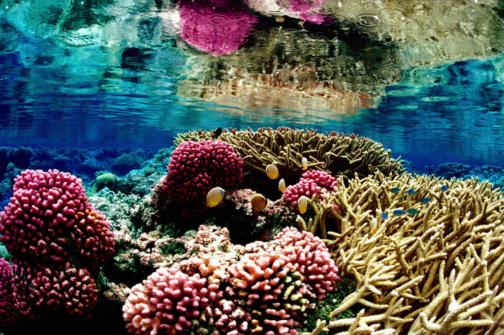
Figure 1. Coral Reef at Palmyra Atoll National Wildlife Refuge. Photo credit: U.S. Fish and Wildlife Service Headquarters/Jim Maragos (CC BY 2.0).

2. Combining tables

In dplyr there are various functions for combining tables.

a) Combining rows with bind_rows

Each animal was given a unique id and weighted. To start with, you have your datasets in two parts: animal_p1 in which you described octopuses and fish; and animal_p2 where you’ve got turtles only.

The datasets are in the same format (columns are in the order; id, animal, weight) so you can simply put them on top of each other with bind_rows().

# 2. Combining tables ----
# a) Combining rows ----

# Firstly view the p1 and p2 datasets, which will appear in your console
animal_p1
animal_p2

# Now, bind them on top of each other
# Adding brackets around the expression prints out the result
(animal <- bind_rows(animal_p1, animal_p2))  # 8 observations

Oh no, it looks like we are missing some observations - we only have 8 in total, and we also can’t find any squids (I remember you told me about seeing them when you had been snorkelling yesterday!). We’ll have to compare your data with your research partner (rp) to find out what is missing.

Your rp’s data are in a separate table (animal_rp) so we will need to compare and hopefully combine them with animal. Together, they can be called relational data - the relations between them are important when we want to connect them. Most importantly, we need a key - a variable which is common for two datasets and thus can be used as a point of reference. This can be the animal’s id because it is unique for each of them. We will use it to combine tables in the following sections.

b) Comparing data with set operations

We’ll first find out how the data tables are different. We can see that both animal and animal_rp have 8 observations in the Environment window in RStudio, but we have no idea if they are the same. While visual comparison would be possible here, if we had thousands of rows of data, that would be much more difficult. Therefore, we can use set operations to compare the data with code.

# b) Set operations ----

setequal(animal_p1, animal_p2)  # FALSE is returned, so the tables are not identical

# Since they differ, let's see how many observations you and your rp have in common.
# You're not creating an object yet so the output will be shown in the console without having to add brackets

intersect(animal, animal_rp)  # 6 observations in common

# View which observations you have and your rp doesn't

setdiff(animal, animal_rp)  # id no. 2 and 5

# Now view which ones your rp has that you don't

setdiff(animal_rp, animal)  # id no. 6 and 10

# Let's now connect them with `union()` but removing any duplicated rows

(animal_weight <- union(animal, animal_rp) %>%
  arrange(id))  # puts the id in numerical order (useful function for rearranging cases!)

Perfect, now we have the animal_weight dataset with 10 unique observations (in the range of 1 to 10). You normally wouldn’t need to use all set operations like above, we could simply use union(). However, the other functions might be useful if you have a different aim of the study (e.g. you could use intersect() to find only observations which are confirmed by two researchers), or simply to get to know your data better.

c) Combining tables with mutating joins

Now, we will want to combine animal_weight with another dataset - animal_meal which contains information on the last meal that you observed for each animal.

# c) Mutating joins ----

animal_meal  # there are 21 observations!

We no longer have the name of the animal, but we still have the key - unique id - based on which we will be able to combine the two tables by adding columns to each other.

Note: if we didn’t have any key, but e.g. we knew that rows in both tables are in the same order (OR the order didn’t matter and we simply wanted to add random meal to each animal), we could use bind_cols(). Here, it would generate various NAs since the number of observations for two tables is not equal.

There are many different functions in dplyr to combine tables, but each is different and might be better suited for your needs. The following are called mutating joins and are used to combine variables from two tables in slightly different ways. Don’t get put off by the number of functions, I have spent quite a lot of time trying to understand them! Hopefully, I will make it easier for you to understand with the diagram (fig. 2) and explanations below.

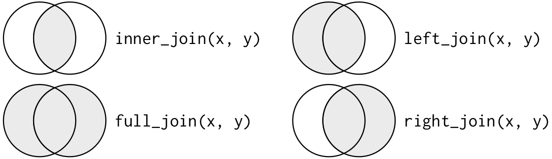
Figure 2. Basic depiction of mutating joins with a Venn diagram. Source: R for Data Science (CC BY-NC-ND 3.0 US).

So each join will return different information. In the case of our ocean animals, we have a table of animal_weight which we checked thoroughly, and now we simply want to add meal information for each individual animal, recognised by its id.

(animal_joined <- left_join(animal_weight, animal_meal,
                            by = c("id" = "IDs")))  # indicate which columns in two tables refer to the same `id` variable

# We can also write it differently by using the pipe operator
(animal_joined <- animal_weight %>%
  left_join(animal_meal, by = c("id" = "IDs")))

What happened here? We used left_join() to keep animal_weight as the “base” to which meal information was added. That way we kept only the 10 animal id’s (from 1 to 10) that we were interested in, and only for them we added meals. We can see that turtle of id == 2 was given <NA> which means that there was no id match in animal_meal.

Note: We have specified that tables should be connected by = c("id" = "IDs") so that RStudio knows what is our key for matching both tables. Since in animal_meal the id column was named IDs, we had to tell RStudio that both tables are describing the same key. But even if both datasets were named id from the beginning, it is always a good practice to specify by = so that we are 100% sure what is happening to our data!

Now, let’s check the other joins!

inner_join(animal_weight, animal_meal, by = c("id" = "IDs"))  # only rows with id's appearing in both tables were left (turtle of id = 2 is now missing)

right_join(animal_weight, animal_meal, by = c("id" = "IDs"))  # we have all meal id's but various NAs for `animal` and `weight` columns were introduced because there was no match for them in `animal_weight`

full_join(animal_weight, animal_meal, by = c("id" = "IDs"))  # all possible id's from both tables are retained and various NAs are introduced

You might have noticed that we could also have used a mutating join full_join() when adding the rows on top of each other in part “a) connect rows of data with bind_rows()”.

full_join(animal_p1, animal_p2, by = c("id", "animal", "weight"))

Yes, that’s perfectly fine! I think it is great to get to know all the functions which might later prove in different contexts. When using full_join() for adding rows on top of each other, remember to always specify all the columns by which the function should join the two tables (otherwise they might be added next to each other instead).

d) Combining tables with filtering joins

Another group of joins which is useful to know about are filtering joins.

# d) Filtering joins ----

semi_join(animal_weight, animal_meal, by = c("id" = "IDs"))  # returns `animal_weight` dataset apart from rows of which `id` is not present in `animal_meal`

anti_join(animal_weight, animal_meal, by = c("id" = "IDs"))  # returns only one row from `animal_weight` of which `id` was not present in `animal_meal`

So, as you have seen with the code above, filtering joins allow you to filter the x dataset based on the matches with y dataset. We’re not going to use them any further, but remember that semi_join() and anti_join() can be useful to identify matches or mismatches in the datasets.

e) Challenge

Well done! You should now have some understanding of the different types of joining tables and of the diverse functions that can be used to do that in R!

Actually, while you were testing all the functions, your research partner collected 10 more observations!

# e) Challenge ----

animal_new <- read.csv("data/animal_new.csv")
str(animal_new)  # check the dataset

Now, take the challenge to create a final_animal table by combining animal_new with your table animal_joined!

animal_final <- animal_joined %>%
  full_join(animal_new,
            by = c("id" = "ID", "animal" = "Animals", "weight", "meal" = "Meal"))

Now let’s visualise what is the meal type and average weight for each animal type you found (fig. 3). If you are not familiar with ggplot2 and you would like to learn to use it, head to the Coding Club tutorial on data visualisation!

# Libraries
library(ggplot2)    # one of the tidyverse packages for beautiful graphs
library(gridExtra)  # for the panel

# Barplot of diet
(barplot <- ggplot(animal_final, aes(animal, fill = meal)) +
  geom_bar(alpha = 0.8) +
  labs(title = "Diversity of meals", x = NULL) +
  scale_fill_brewer(palette = "Set3", type = "seq", na.value = "grey") +
  theme_minimal() +
  theme(plot.title = element_text(size = 14, hjust = 0.5, face = "bold"),
        plot.margin = unit(c(0.5, 0.5, 0.5, 0.5), units = , "cm")))

# Boxplot of weight
(boxplot <- ggplot(animal_final) +
  geom_boxplot(aes(animal, weight, fill = animal), alpha = 0.5, position = "dodge2") +
  scale_y_continuous(limits = c(0, 30)) +
  labs(title = "Mean weights of animals", x = NULL, y = "Weight (kg)") +
  theme_minimal() +
  theme(plot.title = element_text(size = 14, hjust = 0.5, face = "bold"),
        plot.margin = unit(c(0.5, 0.5, 0.5, 0.5), units = , "cm")))

# Combine the plots into one panel
animal_panel <- grid.arrange(barplot, boxplot, ncol = 2)

# Save the panel if you want! You will have to create `images` folder where you've set your working directory (or change filename to "animal_panel.png")
ggsave(filename = "images/animal_panel.png", plot = animal_panel, width = 10, height = 5)

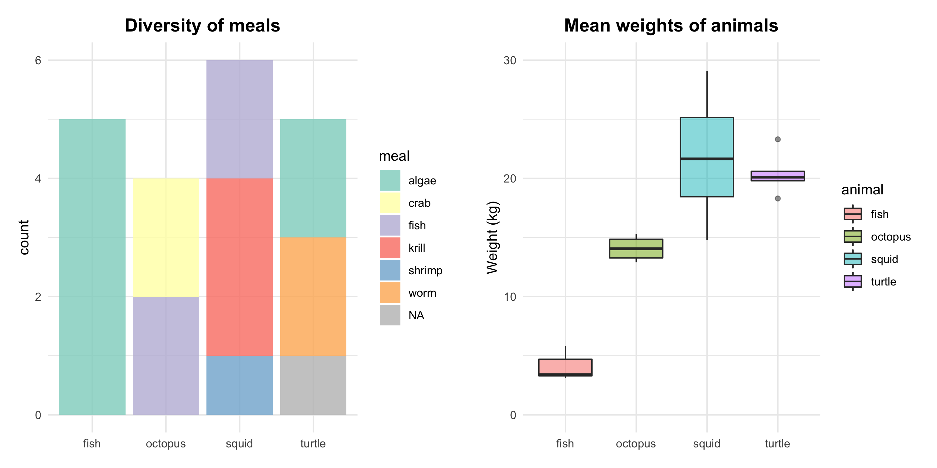
Figure 3. Results of the study on ocean animals. Left: the varying meal types of the ocean animals. Right: significant differences in animals’ weight, with the highest mean for squids and the lowest for fish.

Part II: Oceania LPI data

Now that we know some useful tricks for combining tables, we’ll have a closer look at manipulating variables and cases. As promised, we’ll now get a grasp of real-world dataset - Living Planet data. It might be more complicated because we will be handling thousands of rows of data, but this will give you a great hands-on experience which you can use for your future projects!

We’re going to have a look at Oceania’s marine species populations between 1970 and 2014.

### PART II: OCEANIA LPI DATA ----

# Libraries
# We'll need some extra functions from `tidyverse` package for initial data wrangling, but we will then come back to `dplyr`!
library(tidyr)
library(readr)

# Load the LPI dataset
marine <- read.csv("data/LPI_marine.csv")  # you can also use `readr::read_csv()` - much faster for large files

# Now let's tidy the data a little
marine2 <- marine %>%
  # change to long format with `tidyr::gather()`
  gather(key = year, value = pop, c(25:69)) %>%
  # get rid of X's for year with `readr::parse_number()`
  mutate(year = parse_number(as.character(year)),
         # define `pop` to be numeric, missing data/character entries will become NAs
         pop = as.numeric(pop)) %>%
  # drop all missing values
  drop_na(pop)

# Ignore the warning message on NAs, that's because we kept only numeric values for `pop`

glimpse(marine2)  # have a look at the dataset
View(marine2)  # you can also scroll through the table

We have changed the data to long format so that it is easier to work with (each observation is in a separate row), we also got rid of some X-s for year variable and dropped missing or incorrect values for population variable. We’ll now get to the details of dplyr functions, but if you want to know more on basic data tidying (like changing data to long format), head to the Basic data manipulation tutorial.

Note: in the following sections we’ll try to create as few objects as possible, not to overload your environment in RStudio. To learn different functions, we’ll be using a dplyr function - glimpse(), which is a nice alternative to str() and allows you to view all variables’ names, data type, and some values for each (in a very tidy way!).

3. Manipulating variables

With dplyr, you can easily manipulate variables by extracting entire columns, rename them or create new ones.

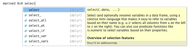
a) Extracting variables: select() and others

Firstly, let’s extract a column which can be transferred into a new vector (with pull()) or a table (with select()).

# 3. Manipulating variables ----
# a) Extracting variables ----

marine2 %>%
  pull(Species) %>%
  glimpse()  # returns a vector of values

marine2 %>%
  select(Species) %>%
  glimpse()  # returns a new table with one column

select() is especially useful because it is quite flexible in its use to create new tables.

We can create a new table with chosen columns and in the preferred order.

# Select only columns you need, in the order you want
marine2 %>%
  select(id, pop, year, Country.list) %>%
  glimpse()

As well as you can give the new names to the columns of the new table.

# Rename columns using the format `new_name = previous_name`
marine2 %>%
  select("Country list" = Country.list,  # you can use names than include spaces or other symbols that can create errors by putting them in `""`
         method = Sampling.method) %>%
  glimpse()

If you want to reorder some columns and leave the rest unchanged, you can use everything().

# Use `everything()` to return all unselected columns
marine2 %>%
  select(id, year, pop, everything()) %>%
  glimpse()  # notice that `id`, `year` & `pop` went to the front but the rest is unchanged

You can also indicate the range of columns you want to keep using star_col:end_col (by using column names or numbers).

# Add ranges of columns with `star_col:end_col`
marine2 %>%
  select(Family:Species, 24:26) %>%
  glimpse()

Delete columns you don’t need with - (remember, if you delete multiple columns use select(-c()) so that - is applied to all of them).

# Delete columns with `-`
marine2 %>%
  select(-c(2:22, 24)) %>%
  glimpse()

Define the chosen columns in a vector beforehand and then recall it with !!.

# Call a vector of column names with `!!`
marine_cols <- c("Genus", "Species", "year", "pop", "id")

marine2 %>%
  select(!!marine_cols) %>%
  glimpse()

Moreover, you can use select() with these functions:

• starts_with("x") matches names starting with “x”
• ends_with("x") matches names ending with “x”
• contains("x") matches names containing “x”

# Choose columns with names starting with "Decimal"
marine2 %>%
  select(starts_with("Decimal")) %>%
  glimpse()

You can also select columns based on their data type using select_if(). The common data types to be called are: is.character, is.double, is.factor, is.integer, is.logical, is.numeric.

marine2 %>%
  select_if(is.numeric) %>%
  glimpse()  # numeric data types only selected (here: integer or double)

You can also mix various ways to call columns within select():

marine2 %>% select(id,  # put id first
                   Class:Family,  # add columns between `Class` and `Family`
                   genus = Genus,  # rename `Genus` to lowercase
                   starts_with("Decimal"),  # add columns starting with "Decimal"
                   everything(),  # add all the other columns
                   -c(6:9, system:Data.transformed)) %>%  # delete columns in these ranges
  glimpse()
# OK, maybe it wasn't the most effective way of reaching the end state here but it proves the point of large flexibility!

Now that we have learned all the varieties of extracting variables with select(), let’s just keep the columns we want to use in further tasks (and do it efficiently!).

# Save a new object `marine3` that we'll keep
marine3 <- marine2 %>%
  select(id, Class, Genus, Species, year, pop,
         location = Location.of.population,
         lat = Decimal.Latitude,
         lon = Decimal.Longitude) %>%
  glimpse()

b) Renaming variables: rename() and others

We still have some uppercase letters in marine3. I prefer to have all variable names in lowercase for higher clarity (and for a lower chance of mistyping them!). Since we didn’t do it with select() when creating marine3, we can now just rename them with rename(), or rename_with().

# b) Renaming variables ----

# Renaming to lowercase
marine3 %>%
  rename(class = Class,
         genus = Genus,
         species = Species) %>%  # renames only chosen columns
  glimpse()

If we just want column names to be changed with a function, we can use rename_with which is useful in this case since we can rename them with tolower.

marine3 %>%
  rename_with(tolower) %>%
  glimpse()
# If you didn't want all of them renamed, you could specify columns with `.cols =`

We could have achieved the same as above by selecting all columns and applying tolower.

marine4 <- marine3 %>%  # let's save this one!
  select_all(tolower) %>%
  glimpse()

If we wanted only some of them renamed and kept, we could have used select_at() which specifies columns with vars().

# Select and rename a couple of columns only
marine3 %>%
  select_at(vars(Genus, Species), tolower) %>%
  glimpse()

You may have noticed that if you knew just one of these functions, you would manage to rename these columns. However, this was just to show you the diversity of dplyr functions which might sometimes cut you a line of code, or make it easier when you want to rename a number of them efficiently. If you’re unsure about any aspect of these functions in a month’s time, e.g. what is this vars() or what is the difference between select_with() or rename_with(), you can always check it easily in RStudio. When you start writing the function, it will give you suggestions what these functions can be - simply put the cursor on the chosen function and you will easily manage!

And remember, these are not complicated and you can usually guess the right function by thinking about the exact action you want to undertake (have a look below!).

These variants are quite flexible, and keep changing for individual functions (e.g. RStudio tells me now that rename_with() has superseded previously used rename_all(), rename_at(), rename_if()). This will happen with time, so stay open-minded about these functions and use help from RStudio to make your code efficient!

c) Making new variables: mutate() and others

The family of mutate() functions can be used to create new variables by applying vectorized functions to entire columns. It’s a yet another amazing function because you can do pretty much everything with it (of course in terms of making new variables)!

Let’s firstly create a genus_species variable by connecting genus and species with an underscore.

# c) Making new variables ----

# New column appears at the end of the table
marine5 <- marine4 %>%
  mutate(genus_species = paste(genus, species, sep = "_")) %>%
  glimpse()

We can also use ifelse() or case_when(), and the logical operators. The mutate() function takes each row of the table and calculates the new value in the new column with the function of our choice!

marine6 <- marine5 %>%
  mutate(region = case_when(lat > 0 & lon >= 0 ~ "NE",
                            lat <= 0 & lon >= 0 ~ "SE",
                            lat > 0 & lon < 0 ~ "NW",
                            lat <= 0 & lon < 0 ~ "SW")) %>%
  glimpse()

unique(marine6$region)  # we've got populations from both sides of equator and meridian 180!

Another function is transmute() which creates the new columns and drops the rest. Let’s use it with the examples of variables added above (genus_species and region).

# A table of only two variables: `genus_species` and `region`
marine4 %>%
  transmute(genus_species = paste(genus, species, sep = "_"),
            region = case_when(lat > 0 & lon >= 0 ~ "NE",
                               lat <= 0 & lon >= 0 ~ "SE",
                               lat > 0 & lon < 0 ~ "NW",
                               lat <= 0 & lon < 0 ~ "SW")) %>%
  glimpse()

Similarly to select(), mutate() also has _at, _all and _if variations. The mechanism is generally the same so we won’t go through all the examples. Let’s just have a look at mutate_at(). We will indicate the variables with vars(), and then change all values for these variables to lowercase. Notice that with the earlier example of lowercase, select() dealt with column names (i.e. changed names to lowercase) while mutate() deals specifically with the values of chosen columns.

# Change values to lowercase
marine6 %>%
  mutate_at(vars(class, genus, location), tolower) %>%
  glimpse()  # column names stayed the same, but individual values within them are lowercase

Apart from mutate(), another way to create new variables can be with add_ functions, e.g. add_column().

# Adding a column (`add_column()` is from a different package - `tibble`)
library(tibble)  # load `tibble` package

marine6 %>%
  add_column(observation_num = 1:4456) %>%  # we gave each row an observation number
  glimpse()

There are also summarising functions count() and tally() which have a mutating variation as add_count() and add_tally(). Here we will see how many unique annual observations we have for each species.

# Summarising functions
marine6 %>%
  select(genus_species, year) %>%
  group_by(genus_species) %>%
  add_tally(name = "observations_count") %>%
  glimpse()

marine6 %>%
  select(genus_species, year) %>%
  # `add_count()` includes the grouping variable (here `genus_species`) inside the function
  add_count(genus_species, name = "observations_count") %>%
  glimpse()

Nice! Now you know quite a variety of possibilities for creating new variables!

4. Manipulating cases

Now, we’ll talk about manipulating cases - so that’s working with rows.

a) Extracting cases: filter() and others

In this section, we’ll talk about how to filter the dataset to return a subset of all rows. We can filter to a specific category or a few categories with, conveniently named, filter().

Table 1. Common logical operators.

The most common use is of == when we want to e.g. filter the table for a specific class or species.

# 4. Manipulating cases ----
# a) Extracting cases ----

# Here we use comparison operator `==`
marine6 %>%
  filter(class == "Mammalia") %>%
  glimpse()  # mammals only

We can also filter it for a few matching values.

# Match one of the specified values with `%in%`
marine6 %>%
  filter(class %in% c("Mammalia", "Aves")) %>%
  glimpse()  # mammals and aves

# Same result as above but using `|`
marine6 %>%
  filter(class == "Mammalia" | class == "Aves") %>%
  glimpse()

Or we can omit some categories with !.

# Omit a category
marine6 %>%
  filter(class != "Actinopteri") %>%
  glimpse()  # all classes but Actinopteri

marine6 %>%
  filter(!class %in% c("Mammalia", "Aves")) %>%
  glimpse()  # remove classes of mammals and aves

We can also filter based on numeric variables.

# Filter numeric variables
marine6 %>%
  filter(pop >= 10 & pop <= 100) %>%
  glimpse()  # observations for population size between 10 and 100

marine6 %>%
  filter(between(pop, 10, 100)) %>%
  glimpse()  # same as above but more aesthetically pleasing!

We can also use filter() to drop NAs.

# Delete NAs from `pop`
marine6 %>%
  filter(!is.na(pop)) %>%
  glimpse()  # there's already none because we deleted them earlier with `mutate()`!

Wow, you can do a lot within this one function! But remember to always understand your specified conditions and how they interact with each other in the function. When using multiple logical operators, you might easily become trapped in too much complexity. In the example below, I will only add brackets to the code but this largely changes the meaning of conditions!

# Be careful with logical operators
marine6 %>%
  filter((class == "Mammalia" | pop > 100) & region != "SE") %>%
  glimpse()  # 38 rows

# Argument 1: class is Mammalia or population is larger than 100
# AND
# Argument 2: in each case the region cannot be SE


marine6 %>%
  filter(class == "Mammalia" | (pop > 100 & region != "SE")) %>%
  glimpse()  # 96 rows!

# Argument 1: class is Mammalia
# OR
# Argument 2: population is larger than 100 and region is not SE

Again, filter() has the _at(), _all(), and _if() variations, but I don’t want to overload you with more examples. These can be however quite useful, especially if you want to e.g. detect strings within the values! I will redirect you to Suzan Baert’s tutorial on filter() where you can find these variations explained very well!

Apart from filter() family, we also have a few other friendly functions to extract cases.

distinct() can be used to drop all duplicated rows (warning: make sure you want to do that, you can check duplicates with base R function duplicated()).

marine6 %>%
  distinct() %>%
  glimpse()  # still 4456 rows so there were no duplicates!

# You can also check a number of distinct rows directly with `n_distinct()` - equivalent of length(unique(x))
marine6 %>%
  n_distinct()  # 4456 distinct rows

slice() can be used to select which rows we want to keep.

marine6 %>%
  select(id:species) %>%  # we'll keep less columns for clarity
  slice(2:4)  # keep only rows 2, 3 and 4! (they get new numbers though - 1, 2, 3)

And top_n() can be used to select and order top entries.

marine6 %>%
  top_n(5, pop) %>%  # 5 highest population values
  glimpse()

b) Adding cases: add_row()

Lastly, if you would like to manually add an observation, you can use add_row(). Although it is actually a function from tibble package, it’s also important to learn!

But first, quick exercise to keep you fresh! Can you take the challenge to create marine7 from marine6 which you will need to complete this section? Create a new table for Chrysophrys auratus population with the id number of 2077. Then, keep only the columns of id, full species name (in Latin!), year of measurement and size of the population.

# b) Adding cases ----

# Create a table for id == "2077"
(marine7 <- marine6 %>%
  filter(id == "2077") %>%
  select(id, genus_species, year, pop))  # we can see 27 observations for 1970-1996

Nice! Now to the new function. Let’s say we wanted to add an observation for the year 1997 at the bottom of the table.

# Add a row at the end
(marine7 %>%
  add_row(id = 2077, genus_species = "Chrysophrys_auratus", year = 1997, pop = 39000))

You can also add a row at a specified location with .before =.

# Add a row at a specified location
(marine7 %>%
  add_row(id = 2077, genus_species = "Chrysophrys_auratus", year = 1969, pop = 39000,
          .before = 1))

Great! Manipulating cases should no longer be a mystery to you :)

5. Extra: Green Sea Turtle population trend

Let’s make use of our LPI dataset and visualise population trends over time of Green Sea Turtle (Chelonia mydas). We won’t go into detail of how to produce this graph, but if you want to learn more on data visualisation, have a look at these Coding Club tutorials: Data vis. 1 & Data vis. 2.

# 5. Extra: Green Sea Turtle population trend ----

marine_final <- marine6 %>%
  filter(genus_species == "Chelonia_mydas") %>%
  # change `id` to factor (otherwise it would display as a continuous variable on the plot)
  mutate(id = as.factor(id))

library(ggplot2)  # you don't have to load it again if you've done it in part 2e

(chelonia_trends <- ggplot(marine_final, aes(x = year, y = pop, colour = location)) +
    geom_point(size = 2, alpha = 0.7) +
    geom_smooth(method = "lm", colour = "black", fill = "lightgrey") +
    scale_x_continuous(limits = c(1970, 2005), breaks = c(1970, 1980, 1990, 2000)) +
    labs(x = NULL, y = "Population count\n",
         title = "Positive trend of Green Sea Turtle population in Australia\n",
         colour = "Location") +
    theme_minimal() +
    theme(plot.title = element_text(size = 14, hjust = 0.5, face = "bold"),
          plot.margin = unit(c(0.5, 0.5, 0.5, 0.5), units = , "cm")))

ggsave(chelonia_trends, filename = "images/chelonia_trends.png", width = 8, height = 6)

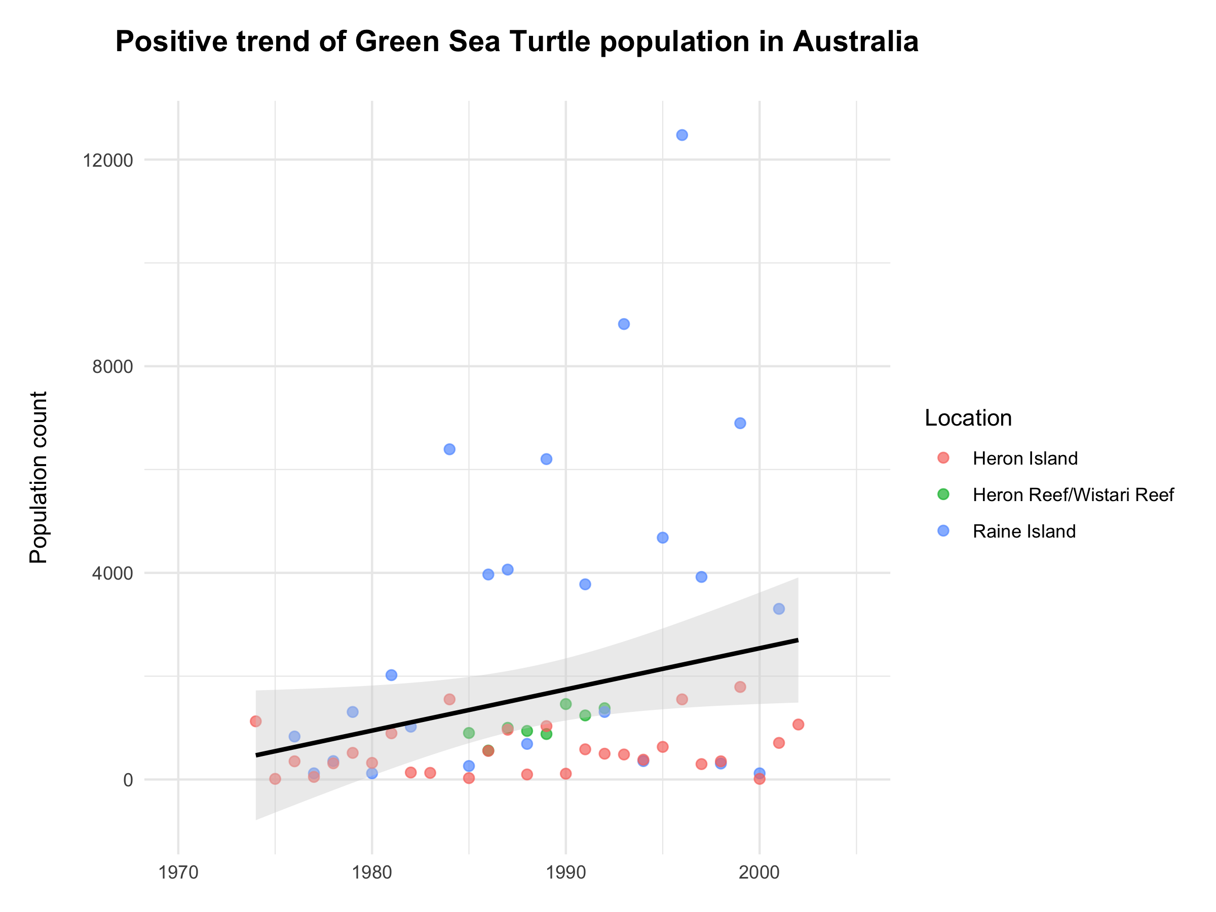
Figure 4. Population trend of Green Sea Turtle seems to be increasing in the past decades. The trend is marked with a bold black line along with an error band (shaded area). Data source: Living Planet Index.

We’re finishing off with a positive message of the increase in the measured Chelonia mydas populations across Australia (fig. 4). I hope you have enjoyed today’s journey with dplyr and will be able to make use of these creative functions in your future data manipulations tasks!

Figure 5. Green Sea Turtle. Photo credit: Kris-Mikael Krister (CC BY 2.0).

Hopefully, you have:

1. Learned about the enormous potential of different dplyr functions and know where to go for more information (check the links throughout the tutorial if you haven’t already!).
2. Learned a range of functions to combine tables.
3. Learned how to be creative and efficient in the manipulation of cases and variables.

And remember, it wasn’t the goal of this tutorial for you to perfectly memorise these functions - you can always go back to the script you wrote today (or this website) and get inspired for any future data manipulation tasks! Alternatively, have a look at RStudio’s Data Transformation Cheatsheet which is a summary of dplyr functions.

If you have any questions or feedback on this tutorial, please feel free to reach out to me on jd.wieczorkowski@gmail.com.