Tutorial Aims:
- Learn to fit simple models on area data
- Learn the basics of geostatistical (marked points) data modelling
- Construct and run more complex spatial models
- Plot spatial predictions and Gaussian random field
Keen to take your analyses and statistical models to the next level? Working with data distributed across space and want to incorporate their spatial structure in your models? If yes, read on and you can jumpstart your spatial modelling journey! This tutorial is meant to be a starting point for anyone interested in spatial modelling, and aims to show the basics of modelling spatial data using R-INLA.
This is by no mean a comprehensive tutorial, and it’s only scratching the surface of what is possible using INLA. However, my main goal with this tutorial is to give you the tools needed to start a basic analysis, in a way that would make more advanced customisation of the model possible (if not easy) using the available resources.
The first and most important concept you need to remember (in my opinion), is the concept of neighbourhood. By Tobler’s first law of geography, “Everything is related to everything else, but near things are more related than distant things, in practice this translate in having neighbours (or individuals from a given species, or entire plots, if you’re an ecologist) that are more similar with each other than individuals that are far away.
INLA explicitly uses neighbouring structures to estimate the spatial autocorrelation structure of the entire dataset. For area data this is relatively straghtforward as there is an explicit neighbouring structure included in the data (areas either share a border or they don’t). For point processes (i.e., when you have just individual points with coordinates), however, we need to create an artificial discretisation of the space to tell the models which points are close to each other and where each new point have explicit neighbours so we can calculate the spatial autocorrelation structure among them. Once you understand this concept, the steps taken to fit a spatial model become logical, as it is just a matter of finding the best way to discretise the space and relate it back to the original dataset.
Analysis of area data (where each polygon has clearly defined neighbours) is generally more straightforward, and that is where we will start in this tutorial and then we will gradually build up the complexity.
This tutorial assumes working knowledge of GLMs and GLMMs, as well as Bayesian statistics and some experience in spatial data manipulation (especially of raster data). Luckily, all these subjects are covered by previous Coding Club tutorials, so check them out! It might also be useful to have a read of our other INLA tutorial, which includes some introduction to the general framework of R-INLA.
The packages
Before going further in the tutorial, it would be good to start downloading the relevant packages (if you don’t have them already). Some of them (R-INLA in particular), might take several minutes, so you might want to do this before starting the tutorial.
# Adding dep = T means you will also install package dependencies
install.packages("RColorBrewer", dep = T)
install.packages("spdep", dep = T)
install.packages("sp", dep = T)
install.packages("rgdal", dep = T)
install.packages("raster", dep = T)

# To download the most recent stable version of the package.
install.packages("INLA",
                 repos = c(getOption("repos"),
                         INLA = "https://inla.r-inla-download.org/R/stable"),
                 dep = T)
The dataset
We will be using two datasets for this practical, derived from my own fieldwork here in Edinburgh. The purpose of the study was to collect fox scats (i.e. faecal marking) in public greenspace around the city of Edinburgh and analyse them for gastrointestinal parasites.
All the files you need to complete this tutorial can be downloaded from this repository. Click on Code/Download ZIP and unzip the folder, or clone the repository to your own GitHub account.
The question
Is the amount of greenspace significantly correlated with:
A) The number of fox scats found?
B) The number of parasite species (species richness) found in each scat?
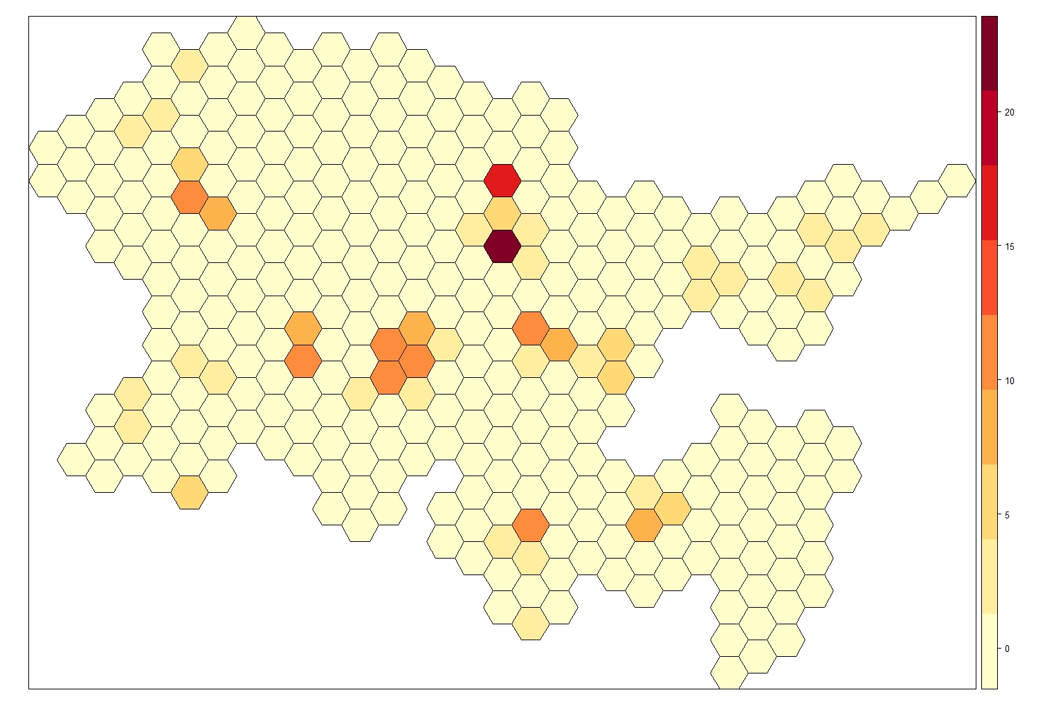
The data I am going to use includes area data of the number of scats found (The hexagonal lattice in the figure) and the point data of the parasite richness we found per sample.

Learn to fit simple models on area data
These kind of data are normally found in epidemiological, ecological or social sciences studies. In brief, the data report a value (often it’s the number of cases of a disease) per area, which could be an administrative district, such as a post-code area, council area, region and so on. The main characteristic of area data is that there are explicit neighbours for each area, which makes computing the autocorrelation structure much easier. A special subset of area data are lattice data, which reports area data from a regular grid of cells (like what we have here). This type of area data is genrally preferable as the space is split in more comparable areas and the space discretisation is more even. However, having this kind of area data is rare, as lattice data are generally constructed specifically from points (in which case it would be best to use the points directly), while real area data generally are derived from surveys done at administrative district levels, which are not regular in shape by nature.
Modelling area data in INLA is relatively straightforward (at least compared to point datasets). This is due to the fact that the areas already have explicit neighbours (you can tell just looking at the figure which cells are next to which others). This means that all we need to do is to translate this into an adjacency matrix which specifies the neighbouring system of our dataset in a way that INLA can understand, then we can fit the model straight away (this is firmly NOT the case with point datasets).
The aim of this section is to carry out a spatial analysis on area data. Here, we are going to test the hypothesis that a higher greenspace ratio (a higher percentage of green areas) is associated with a higher number of scats found. We are going to use a dataset I have modified for the purpose of this tutorial. The data refer to the number of fox scats found in the city of Edinburgh during a 6 months survey of every public green area in the city.
To do so, I have constructed a lattice that covers the study area, and for each zone recorded the number of scats found, along with the greenspace ratio, calculated using the Greenspace Dataset from Edina Digimap.
# Load the lattice shapefile and the fox scat data
require(sp)  # package to work with spatial data
require(rgdal)  # package to work with spatial data

# Fox lattice is a spatial object containing the polygons constructed on the basis of the data
# (normally you would use administrative district)
Fox_Lattice <- readOGR("Fox_Lattice/Fox_Lattice.shp")

#Warning message:
#In readOGR("Fox_Lattice/Fox_Lattice.shp") : Z-dimension discarded
# Ignore this warning message, this is showing since there is not a z-value assigned to each cell (we have attached our response value as a data frame instead)

require(RColorBrewer)
# Create a colour palette to use in graphs
my.palette <- brewer.pal(n = 9, name = "YlOrRd")

# Visualise the number of scats across space
spplot(obj = Fox_Lattice, zcol = "Scat_No",
       col.regions = my.palette, cuts = 8)
As mentioned previously, INLA needs to know which areas are neighbouring, so it can compute the spatial autocorrelation structure, we do that by computing the adjacency matrix.
# We can extract the data frame attached to the shape (file extensioon shp) object
Lattice_Data <- Fox_Lattice@data
str(Lattice_Data)
require(spdep) # a package that can tabulate contiguity in spatial objects, i.e., the state of bordering or being in contact with something
require(INLA) # for our models!
# Specify the adjacency matrix
Lattice_Temp <- poly2nb(Fox_Lattice) # construct the neighbour list
nb2INLA("Lattice.graph", Lattice_Temp) # create the adjacency matrix in INLA format
Lattice.adj <- paste(getwd(),"/Lattice.graph",sep="") # name the object
inla.setOption(scale.model.default = F)
H <- inla.read.graph(filename = "Lattice.graph") # and save it as a graph
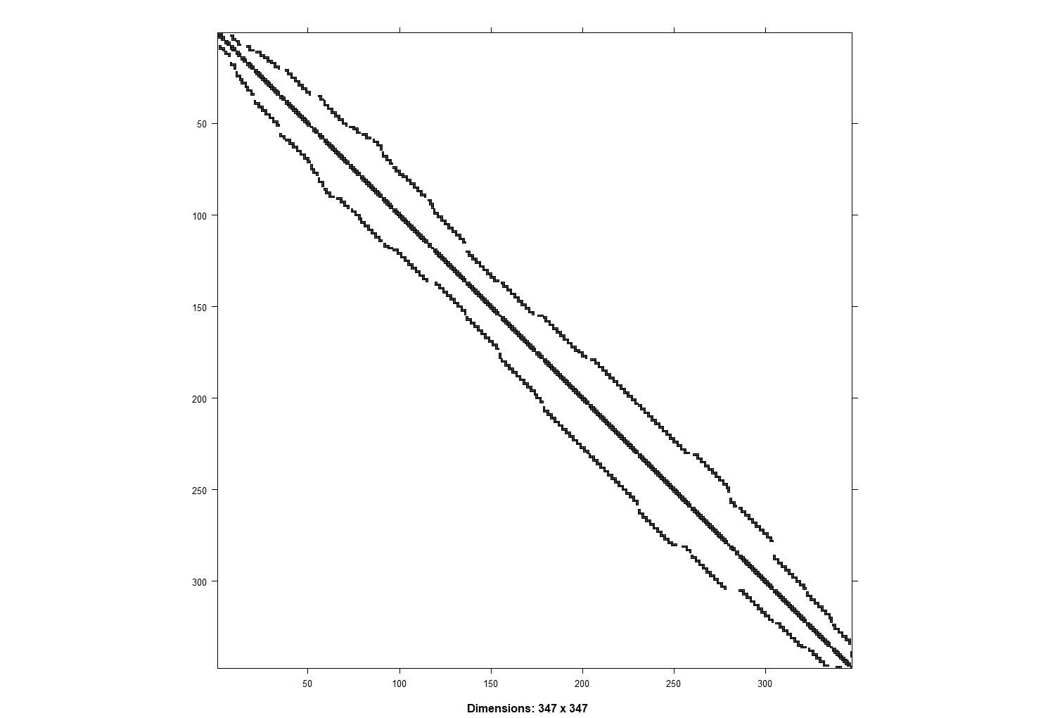
# Plot adjacency matrix
image(inla.graph2matrix(H), xlab = "", ylab = "")
This matrix shows the neighbouring for each cell. You have the cell numerical ID (ZONE_CODE) on both axis and you can find which cells they are neighbouring with (plus the diagonal which means that the cells neighbour with themselves). For example you can trace with your eyes cell number 50 and see its neighbours (cells 49 and 51). Each line will have up to 6 neighbours (hexagons have 6 edges), corresponding to the number of neighbours of the lattice cell. Note that in this case the cells were already sorted in alphabetical order so they are only adjacent to ones with a similar name, so you have a clump of adjacent cells around the diagonal line. When using administrative districts this matrix will likely be messier.
We also need to specify the model formula. This model will test whether there is a linear effect of greenspace ratio (GS_ratio) on the number of fox scats found in each area across Edinburgh. We will do the model formula first, which doesn’t actually run our model, and we will do the running part in the next step.
formula <- Scat_No ~ 1 + GS_Ratio + # fixed effect
  f(ZONE_CODE, model = "bym",       # spatial effect: ZONE_CODE is a numeric identifier for each area in the lattice  (does not work with factors)
    graph = Lattice.adj)            # this specifies the neighbouring of the lattice areas
NOTE: The spatial effect is modelled using the BYM (Besag, York and Mollie’s model) is the model type usually used to fit area data. CAR (conditional auto-regressive) and besag models are other options, but here we will focus on BYM since that is appropriate way to model the spatial effect when working with area data. Now we are ready to run our model!
# Finally, we can run the model using the inla() function
Mod_Lattice <- inla(formula,
                    family = "poisson",  # since we are working with count data
                    data = Lattice_Data,
                    control.compute = list(cpo = T, dic = T, waic = T))
# CPO, DIC and WAIC metric values can all be computed by specifying that in the control.compute option
# These values can then be used for model selection purposes if you wanted to do that

# Check out the model summary
summary(Mod_Lattice)
We’ve now ran our first INLA model, nice one!
In the output you can find some general information about the model: the time it took to run, a summary of the fixed effects, and model selection criteria (if you have specified them in the model), as well as the precision for any random effects (in this case just our spatial component ZONE_CODE). It is important to remember that INLA works with precision (tau = 1/Variance), so higher values of precision would correspond to lower values of variance.
We can see that GS_Ratio has a positive effect on the number of scats found (the 0.025q and 0.075 quantiles do not cross zero so this is a “significant” positive effect), and that the iid (random factorial effect) of ZONE_CODE id has a much lower precision than the spatial effect, which means that using ZONE_CODE as a standard factorial random effect would probably suffice in this case.
Setting priors
We can also set priors for the hyperparameters (the parameters of the prior distribution) by specifying them in the formula. INLA works with precision (tau = 1/Variance) so a very low precision corresponds to a very high variance by default. Keep in mind that the priors need to be specified for the linear predictor of the model (so they need to be transformed according to the data distribution) in this case they follow a log gamma distribution (since it’s a Poisson model).
formula_p <- Scat_No ~ 1 + GS_Ratio +
  f( ZONE_CODE, model = "bym",
     graph = Lattice.adj,
     scale.model = TRUE,
     hyper = list(
       prec.unstruct = list(prior = "loggamma", param = c(1,0.001)),   # precision for the unstructured effect (residual noise)
       prec.spatial =  list(prior = "loggamma", param = c(1,0.001))    # precision for the spatial structured effect
       )
     )

Mod_Lattice_p <- inla(formula_p,
                    family = "poisson",
                    data = Lattice_Data,
                    control.compute = list(cpo = T)
                  )

summary(Mod_Lattice_p)

# We can extract the summary of the fixed effects (in this case only GS)
round(Mod_Lattice$summary.fixed, 3)
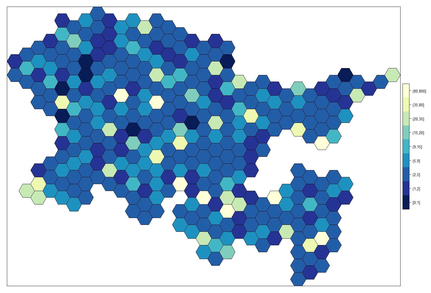
The posterior mean for the random (spatial) effect can also be computed and plotted overlayed to the lattice. To do so, we need to extract the posterior mean of the spatial effect for each of the cells in the lattice (using the emarginal() function) and then add it to the original shapefile so we can map it.
This represents the distribution in space of the response variable, once you accounted for the covariates included in the model. Think of it as the “real distribution” of the response variable in space, according to the model (obviously this is only as good as the model we have and will suffer if the estimation are poor, we have missing data or we failed to include an important covariate in our model).
First we select the marginal posterior distributions of the spatial random effect for each area using the Nareas index, then we use lapply() to calculate the value of the posterior mean of the spatial random effect (zeta) from the marginal distributions for each #area (we exponentiate the distibutions to convert them into real numbers, as the output of the model is expressed in the linear predictor scale of the model which was a log scale).
# Calculating the number of areas
Nareas <- length(Lattice_Data[,1])

# select the posterior marginal distribution for each zone
# these correspond to the first 347 (number of cells) items of the marginal distribution for the spatial random effect (zeta)
zone.index <- Mod_Lattice$marginals.random$ZONE_CODE[1:Nareas]
# exponentiate each of the zone marginals to return it to its original values (remember that this is a poisson model so all the components of the model are log-transformed)
zeta <- lapply(zone.index,function(x) inla.emarginal(exp,x))

zeta.cutoff <- c(0, 1, 2, 5, 9, 15, 20, 35, 80, 800)   # we make a categorisation to make visualisation easier
cat.zeta <- cut(unlist(zeta),
                breaks = zeta.cutoff,
                include.lowest = TRUE)

# Create a dataframe with all the information needed for the map
maps.cat.zeta <- data.frame(ZONE_CODE = Lattice_Data$ZONE_CODE,
                            cat.zeta = cat.zeta)

# Create a new polygon from Fox_Lattice and add the value of the posterior mean
Fox_Lattice_post <- Fox_Lattice
data.fox.post <- attr(Fox_Lattice_post, "data")
attr(Fox_Lattice_post, "data") <- merge(data.fox.post,
                                       maps.cat.zeta,
                                       by = "ZONE_CODE")
Now we are ready to make a colour palette and make our map!
my.palette.post <- rev(brewer.pal(n = 9, name = "YlGnBu"))
spplot(obj = Fox_Lattice_post, zcol = "cat.zeta",
       col.regions = my.palette.post)
Similarly, we can plot the uncertainty associated with the posterior mean. As with any modelling, important to think not just about the mean, but how confident we are in that mean.
a <- 0
prob.zone <- lapply(zone.index, function(x) {1 - inla.pmarginal(a, x)})

prob.zone.cutoff <- c(0, 0.1, 0.3, 0.4, 0.5, 0.6, 0.7, 0.8, 0.9, 1)
cat.prob.zone <- cut(unlist(prob.zone),
                    breaks = prob.zone.cutoff,
                    include.lowest = T)

# Create a new polygon from Fox_Lattice and add the value of the posterior sd
maps.cat.prob.zone <- data.frame(ZONE_CODE = Lattice_Data$ZONE_CODE,
                                cat.prob.zone = cat.prob.zone)

Fox_Lattice_var <- Fox_Lattice
data.fox.var <- attr(Fox_Lattice_var, "data")
attr(Fox_Lattice_var, "data") <- merge(data.fox.var,
                                       maps.cat.prob.zone,
                                       by = "ZONE_CODE")

my.palette.var <- brewer.pal(n = 9, name = "BuPu")
spplot(obj = Fox_Lattice_var, zcol = "cat.prob.zone",
       col.regions = my.palette.var, add = T)
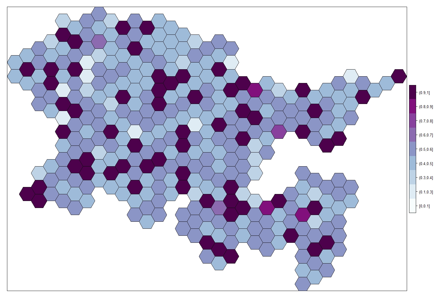
Note that the posterior mean is highest where we have the higher level of uncertainty. We have some area where the response variable reaches really high numbers, this is due to missing GS data in this areas (GS=0), so the model compensates for it; however, these are the areas where we also have the highest uncertainty, because the model is unable to produce accurate estimates.
Learn the basics of geostatistical (marked points) data modelling
For this analysis, we will be using geostatistical data, also known as marked points. This is one of the most common type of spatial data. It includes points (with associated coordinates), which have a value attached, which is generally the measurement of the response variable we are interested here. The idea is that these points are the realisation of a smooth spatial process that happens everywhere in space, and the points are just samples of this process (we will never be able to sample the entire process as there are infinite points in the continuous space).
A classic example would be soil Ph: this is a property of the soil and it exists everywhere, but we will only measure it at some locations. By linking the values we have collected with other measurements we could find out that soil Ph is dependent on precipitation level, or vegetation type, and (with enough information) we could be able to reconstruct the underlying spatial process.
We are generally interested in understanding the underlying process (which variable influences it? how does it change in space and time?) and to recreate it (by producing model predictions).
In this example, we are going to be using the same points I used to generate the dataset for the spatial data (the Edinburgh fox scats), but we will be looking at the number of parasites species (Spp_Rich) found in each scat. The dataset include the location of each point (each one a scat found during the survey), but what we are interested in modelling here is the number of parasite species found in each scat. This means that each point in the dataset has a value attached (a mark, hence the name marked point process), which is what we are interested in modelling.
In this case we do not have explicit neighbours for the points, so we will need to construct an artificial discretisation of the space and tell INLA the neighbouring structure of the discretisation.
The dataset also contains a number of other variables associated with each sample:
- JanDate (the date when the sample was collected)
- Site (which park was it collected from),
- Greenspace variability (
GS_Var) which is a categorical variable measuring the number of different greenspace types (Low, Med, High)
In this case we are going to model the species richness of gastrointestinal parasites as a function of greenspace ratio, while taking into account both the spatial effect and the other covariates mentioned just above.
Point_Data <- read.csv("Point_Data.csv")
str(Point_Data)
When transforming the point dataset into a spatial object, we need to specify a Coordinate Reference System (CRS). The coordinates for this dataset are expressed in Easting / Northing and it’s projected using the British National Grid (BNG). This is important in case you are using multiple shapefiles which might not be in the same coordinate system, and they will have to be projected accordingly.
NOTE: The choice of CRS should be done on the basis of the extent of the study area.
- Small areas - For small areas (such as this), Easting-Northing coordinate systems are best. They effectively express the coordinates on a flat surface (which does not take into account the globe curvature and consequent modification of the projection shape).
- Medium-sized studies - We should use Latitude-Longitude for medium-sized studies (country level/ multi country levels), as this will take into account a more realistic shape of the map.
- Continental and global-scale studies - Finally, for studies conducted at continental and global scale, we should use radians and fit the mesh taking into account the curvature of the globe.
The type of coordinates is important as several steps in the code are unit-specific and should be modified accordingly. I will point them out as they come up. To illustrate this concept, I will plot the points against the shapefile of Scotland, derived from GADM website (an excellent source for administrative district shapefiles), which is mapped using Lat-Long.
require(rgdal)
# First, we need the coordinates of the points
Loc <- cbind(Point_Data$Easting, Point_Data$Northing)
# Then we can transform our dataset in a spatial object (a spatial point dataframe)
Fox_Point <- SpatialPointsDataFrame(coords = Loc, data = Point_Data, match.ID = T,
proj4string = CRS("+proj=tmerc +lat_0=49 +lon_0=-2 +k=0.9996012717 +x_0=400000 +y_0=-100000 +ellps=airy +units=m +no_defs"))
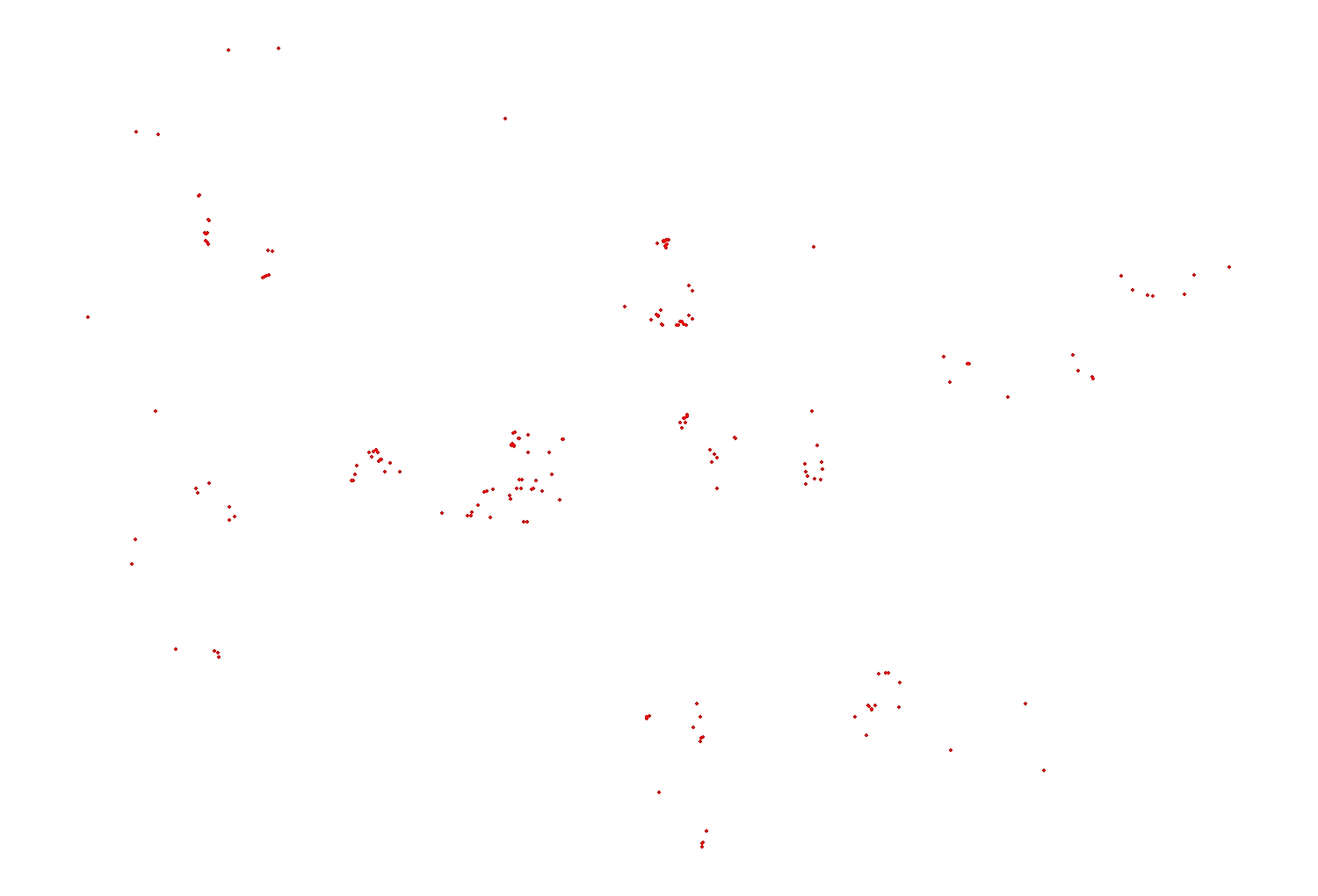
par(mfrow = c(1,1), mar = c(1,1,1,1))
plot(Fox_Point, col = 2, pch = 16, cex = 0.5)
# Load the UK shapefile and subset the Scotland polygon
UK_Shape <- readOGR(dsn = "United Kingdom", layer = "gadm34_GBR_1")
Scot_Shape <- UK_Shape[UK_Shape$NAME_1 == "Scotland",]
# Using the proj4string() function we can check the projection of the shapefile
proj4string(Scot_Shape)
# You should see "+proj=longlat +datum=WGS84 +no_defs +ellps=WGS84 +towgs84=0,0,0"
This is the standard latitude/longitude coordinate system, which is projected in a geodesic system (taking into account the curvature of the globe). Most shapefiles (especially at country level) will use this coordinate system. This Cheatsheet provides more context and explains how to specify the right coordinate system using R notation.
Trying to plot both our points and our shapefile in the same map will not work as they cannot be plotted in their coordinates are expressed in different systems.
plot(Fox_Point, col = 2, pch = 16, cex = 0.5)
plot(Scot_Shape, add = T)
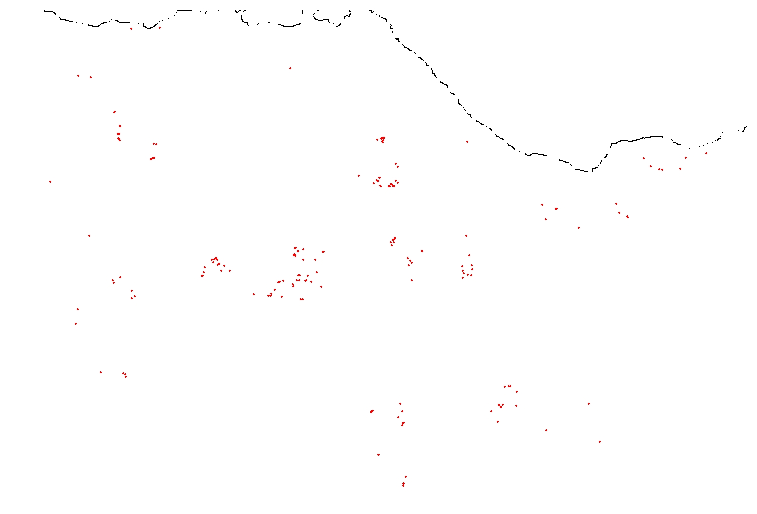
However, if we change the transform the CRS of Scot_Shape using the spTransform() function, we can correctly map correctly the fox scats and the Scotland shapefile together.
foxcrs <- CRS("+proj=tmerc +lat_0=49 +lon_0=-2 +k=0.9996012717 +x_0=400000 +y_0=-100000 +ellps=airy +units=m +no_defs")

Scot_Shape_BNG <- spTransform(Scot_Shape, foxcrs)

plot(Fox_Point, col = 2, pch = 16, cex = 0.5)
plot(Scot_Shape_BNG, add = T)
Now that the data is properly loaded, we can start putting together all the components required by a geostatistical INLA model. We’ll start fitting just a simple base model with only an intercept and spatial effect in it and build up complexity from there.
The absolutely essential component of a model are:
- The mesh
- The projector matrix
- The correlation structure specifier (spde)
- The formula
The Mesh
Unlike the area data, point data do not have explicit neighbours and thus we would have to calculate the autocorrelation structure between each possible point existing in space, which is obviously imposssible. For this reason, the first step is to discretise the space to create a mesh that would create artificial (but useful) set of neighbours so we could calculate the autocorrelation between points. INLA uses a triangle mesh, because is much more flexible and can be adapted to irregular spaces. There are several options that can be used to adjust the mesh.
I will not spend a lot of time explaining the mesh as there are a number of excellent tutorials that do a much better job than I could (check out this one for example), and I find defining the mesh is the easiest part of this INLA modelling process!
# Now we can construct the mesh around our points
Mesh1 <- inla.mesh.2d(Loc,
                      max.edge = c(500))       # this part specify the maximum lenght of the triangle edge.
                                               # THIS NEEDS TO BE SPECIFIED IN COORDINATE UNITS (in this case this would be in metres)
Mesh2 <- inla.mesh.2d(Loc,
                      max.edge = c(900, 2000)) # We can also specify an outer layer with a lower triangle density where there are no points to avoid edge effect

Mesh3 <- inla.mesh.2d(Loc,
                      max.edge = c(900, 2000),
                      cutoff = 500)            # The cutoff is the distance at which two points will be considered as one. Useful for dataset with a lot of points clamped together

Mesh4 <- inla.mesh.2d(Loc,
                      max.edge = c(900, 2000),
                      cutoff = 500,
                      offset = c(1000, 1000))    # The offset control the extension of the two layer (high and low triangle density)
Ideally, we aim to have a regular mesh with an inner layer of triangles, without clumping and with a smooth, lower density of triangles on the outer layer.
par(mfrow = c(2,2), mar = c(1,1,1,1))
plot(Mesh1,asp = 1, main = "")
points(Loc, col = 2, pch = 16, cex = 0.1)

plot(Mesh2,asp = 1, main = "")
points(Loc, col = 2, pch = 16, cex = 0.1)

plot(Mesh3,asp = 1, main = "")
points(Loc, col = 2, pch = 16, cex = 0.1)

plot(Mesh4,asp = 1, main = "")
points(Loc, col = 2, pch = 16, cex = 0.1)
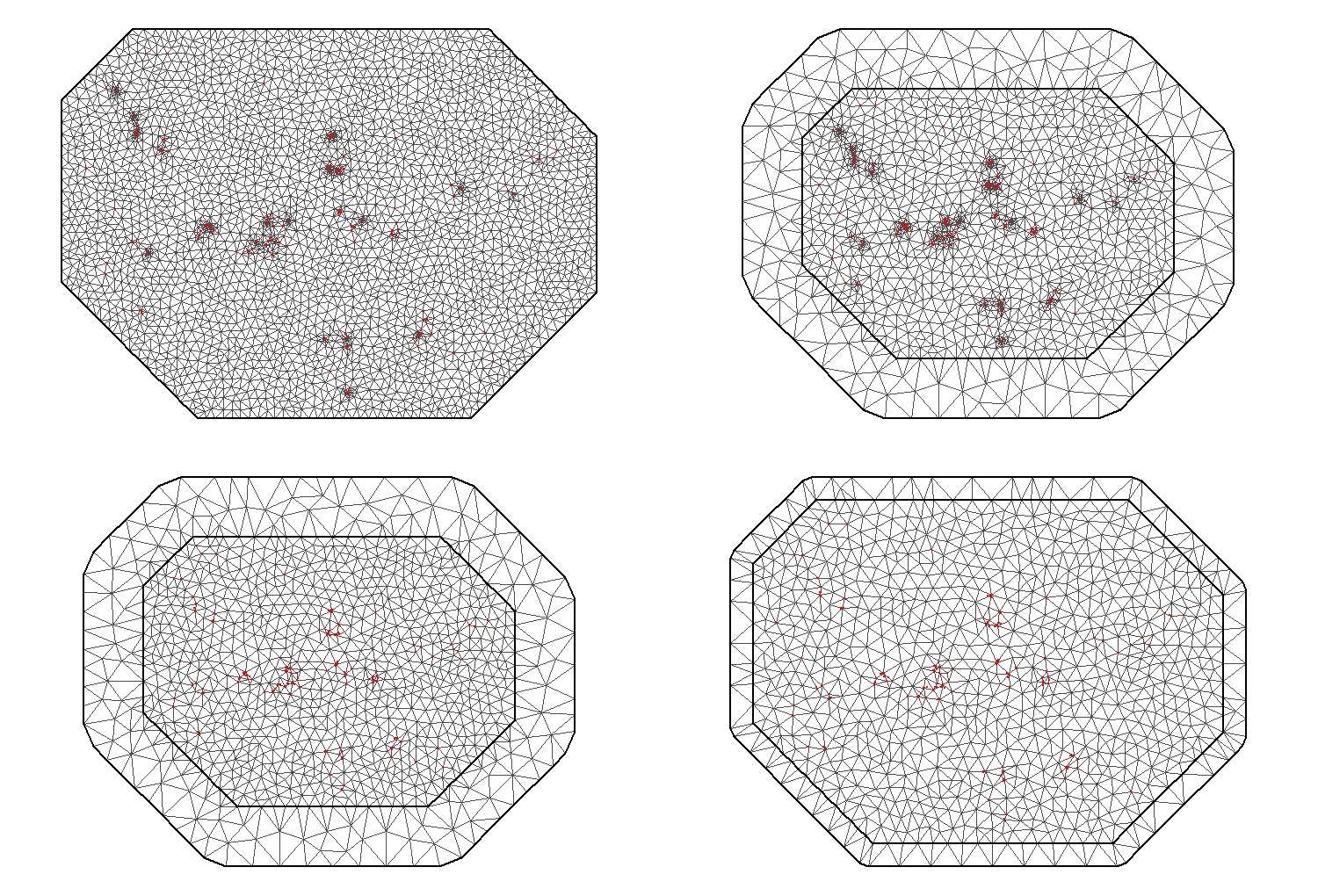
The third Mesh seems the most regular and appropriate for this dataset.
par(mfrow = c(1,1), mar = c(1,1,1,1))
plot(Mesh3,asp = 1, main = "")
points(Fox_Point, col = 2, pch = 16, cex = 1)
plot(Scot_Shape_BNG, add=T)
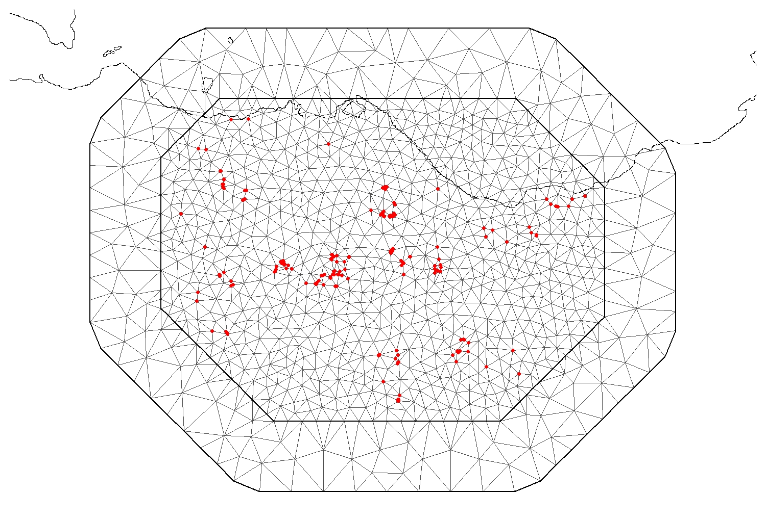
NOTE: You can see that the mesh extends past the coastline into the sea. Since we are trying to evaluate the effect of greenspace ratio on the parasite species of foxes, it makes no sense to include area that are part of the sea in the mesh. There are two possible solutions: the first is to run the model using this mesh and then simply ignore the results the model provides for the sea area. The second is to modify the mesh to reflect the coastline.
Keep in mind that you can either use shapefiles or create nonconvex hulls around the data and use those shapes to create bespoke meshes. Check out the Blangiardo & Cameletti book(chapter 6) for more exhaustive examples.
Projector matrix
Now that we have constructed our mesh, we need to relate the data points to the mesh vertices. The projector matrix provides the model with the neighborhood structure of the dataset using the mesh vertex as explicit neighbours
As mentioned before, geostatistical data do not have explicit neighbours, so we need to artificially discretise the space using the mesh. The projector matrix projects the points onto the mesh where each vertex has explicitly specified neighbours. If the data point falls on the vertex (a vertex is each angular point of a polygon, here a triangle), then it will be directly related to the adjacent vertices (like the blue point in the figure). However, if the datapoints falls within a mesh triangle (dark red point), its weight will be split between the tree vertices according to the proximity of the to each vertex (the red, orange and yellow points with the dark border). The original data point will then have a larger number of “pseudo-neighbours” according to the neighbours of vertices defining the triangles, weighted in a similar manner than those vertices (however, the total weight of each datapoint will always be one.
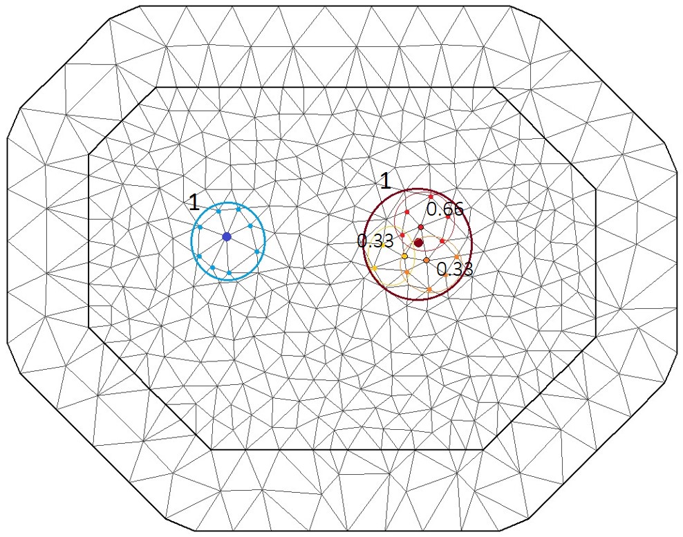
The projector matrix automatically computes the weight vector for the neighbourhood of each point and is calculated by providing the mesh and the locations of the datapoints to the inla.spde.make.A() function.
A_point <- inla.spde.make.A(Mesh3, loc = Loc)
dim (A_point)
# [1] 223 849    # Number of points  # Number of nodes int he mesh
SPDE
The SPDE (Stochastic Partial Differential Equation) is the mathematical solution to the Matérn covariance function and it is effectively what allows INLA to efficiently compute the spatial autocorrelation structure of the dataset at the mesh vertices. It calculates the correlation structure between the vertices of the mesh (which will then be weighted by the vectors calculated using the projector matrix to calculate the correlation matrix applicable to the actual dataset).
spde1 <- inla.spde2.matern(Mesh3,
                            alpha = 2) # alpha is 2 by default, for most models this can be left as it is (needs to be adjusted for 3D meshes)

spde1$n.spde
#[1] 849   # the dimension of the spde is the same as the mesh vertices
Fitting a basic spatial model
We will first fit a model only including an intercept and the spatial effect to show how to code this. This model is simply testing the effect of the spatial autocorrelation on the parasite species richness, without including any other covariate.
One thing to keep in mind is that INLA syntax codes nonlinear effects using the format f(Covariate Name, model = Effect Type). In the case of the spatial effect, the model name is the name you assigned to the SPDE (spde1 in this case). Stay tuned for other type of nonlinear effects coming up later in the tutorial!
#First, we specify the formula
formula_p1 <- y ~ -1 + Intercept +
  f(spatial.field1, model = spde1)       # this specifies the spatial random effect. The name (spatial.field1) is of your choosing but needs to be the same you will include in the model
We have our formula and we’re ready to run the model!
# Now we can fit the proper model using the inla() function
Mod_Point1 <- inla(formula_p1,
                data = list( y = Point_Data$Spp_Rich,         # response variable
                            Intercept = rep(1,spde1$n.spde),   # intercept (manually specified)
                            spatial.field1 = 1:spde1$n.spde),  # the spatial random effect (specified with the matern autocorrelation structure from spde1)
                control.predictor = list( A = A_point,
                                          compute = T),       # this tells the model to compute the posterior marginals for the linear predictor
                control.compute = list(cpo = T))
Now that the model has ran, we can explore the results for the fixed and random effects.
# We can access the summary of fixed (just intercept here) and random effects by using
round(Mod_Point1$summary.fixed,3)
round(Mod_Point1$summary.hyperpar[1,],3)
We can also compute the random term variance by using the emarginal() function (remember that INLA works with precisions so we cannot directly extract the variance).
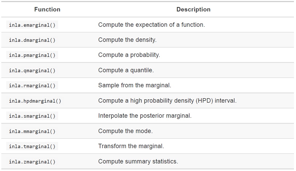
NOTE: INLA offers a number of functions to manipulate posterior marginals. We are only going to use the emarginal() (which computes the expectations of a function and is used, among other things, to transform precision to variance) for this tutorial, but it is worth knowing that there is a full roster of function for marginal manipulation, such as sampling from the marginals, transforming them or computing summary statistics.
Back to extracting our random term variance now.
inla.emarginal(function(x) 1/x, Mod_Point1$marginals.hyper[[1]])

# In order to extract the relevant information on the spatial field we will need to use the inla.spde2.result() function
Mod_p1.field <- inla.spde2.result(inla = Mod_Point1,
                                 name = "spatial.field1", spde = spde1,
                                 do.transf = T)     # This will transform the results back from the internal model scale

names(Mod_p1.field) # check the component of Mod_p1.field
The two most important things we can extract here are the range parameter (kappa), the nominal variance (sigma) and the range (r, radius where autocorrelation falls below 0.1)). These are important parameters of the spatial autocorrelation: the higher the Kappa, the smoother the spatial autocorrelation structure (and the highest the range). Shorter range indicates a sharp increase of autocorrelation between closely located points and a stronger autocorrelation effect.
inla.emarginal(function(x) x, Mod_p1.field$marginals.kappa[[1]])             #posterior mean for kappa
inla.hpdmarginal(0.95, Mod_p1.field$marginals.kappa[[1]])                    # credible intervarls for Kappa

inla.emarginal(function(x) x, Mod_p1.field$marginals.variance.nominal[[1]])  #posterior mean for variance
inla.hpdmarginal(0.95, Mod_p1.field$marginals.variance.nominal[[1]])         # CI for variance

inla.emarginal(function(x) x, Mod_p1.field$marginals.range.nominal[[1]])     #posterior mean for r (in coordinates units)
inla.hpdmarginal(0.95, Mod_p1.field$marginals.range.nominal[[1]])            # CI for r
Construct and run more complex spatial models
Normally we are interested in fitting models that include covariates (and we are interested in how these covariates influence the response variable while taking into account spatial autocorrelation. In this case, we need to add another step in the model construction.
We will retain the same mesh we used before (Mesh3), and the projector matrix (A_point), and we will continue from there.
I am going to mention in passing a variety of custumisations to the model (such as spatio-temporal modelling). While I think it’s beyond the scope of this practical for me to go into details for the many possible customisations, you can find a lot of useful examples (and code) in the recent book “Advanced Spatial Modeling with Stochastic Partial Differential Equations Using R and INLA”, which also includes really useful tables of customisation options for the inla() function.
We are now going to expand our model to include all the available components:
- The mesh
- The projector matrix
- The correlation structure specifier (SPDE), including PC priors on the spatial structure
- The spatial index
- The stack
- The formula
Specify PC priors
We can provide priors to the spatial term. A special kind of priors (penalised complexity or pc priors) can be imposed on the SPDE. These priors are widely used as they (as the name suggests) penalise the complexity of the model. In practice they shrink the spatial model towards the base model (one without a spatial term). To do so we apply weakly informative priors that penalise small ranges and large variances.
Check out the Fulgstag et al (2018) paper for a more detailed theoretical explanation of how PC priors work.
spde.pc   <- inla.spde2.pcmatern(Mesh3,                      # inla.spde2.pcmatern() instead of inla.spde2.matern()"
                                 prior.range = c(500,0.01),  # the probability that the range is less than 300 (unit) is 0.01. The range here should be rather large (compare to the dataset extension)
                                 prior.sigma = c(1, 0.01))   # the probability that variance (on the log scale) is more that 1 is 0.01
Spatial index
One useful step includes constructing a spatial index. This will provide all the required elements to the SPDE model. This is not strictly necessary, unless you want to create multiple spatial fields (e.g. year-specific spatial fields). The number of replicates will produce iid independent, identically distributed replicates (the variance will be equally distributed between the levels, which is equivalent to a GLM standard factorial effect), while the number of groups will produce dependent replicates (each level of the group will depend from the previous/following one).
Shown beneath are the default settings for the index (no replicates or groups are specified):
s.index <- inla.spde.make.index(name = "spatial.field2",
                                n.spde = spde.pc$n.spde,
                                n.group = 1,
                                n.repl = 1)
The Stack
The stack has become infamous for being particularly fiddly to handle, but in short, it provides all the elements that are going to be used in the model. It includes the data, the covariates (including linear and non-linear ones), and the index for each of them. One thing that is useful to remeber is that the stack does NOT automatically include an intercept, so this will need to be specified explicitly.
# We need to limit the number of levels that greeen space (GS_Ratio) has. This way, GS can only have 100 levels between 0 and 100
Point_Data$GS_Ratio2 <- round(Point_Data$GS_Ratio*100)

StackEst <- inla.stack(data = list(y = Point_Data$Spp_Rich),               # First off, the response variable

                        A = list(A_point, 1),                              # Then the projector matrix (for the spatial effect) and a linear vector (1) for the other effects

                        effects = list(c(s.index, list(Intercept = 1)),    # The effects are organised in a list of lists. spatial effect and intercept first

                                       list(GS_Var = Point_Data$GS_Var,    # Then all the other effects. We will specify the type of effect using the formula
                                            GS_Ratio = Point_Data$GS_Ratio2,
                                            JanDate = Point_Data$JanDate,
                                            SiteID = Point_Data$Site)),

                        tag="Est")                                          # The tag specify the name of this stack
NOTE: The intercept in this case is fit to be constant in space (it is fit together with the spatial effect, which means that it is always 1 at each of the n.spde vertices of the mesh). This is not necessarily the case, if you want to fit the intercept to be constant through the dataset (and hence be affected by the spatial effect), you can code it together with the list of the other covariates, but keep in mind that then you will need to specify intercept as Intercept = rep(1, n.dat), where n.dat is the number of datapoints in the dataset (rather then the number of mesh vertices).
Fitting the model
In the formula, we specify what kind of effect each covariate should have. Linear variables are specified in a standard GLM way, while random effects and non-linear effects need to be specified using the f(Cov Name, model = Effect Type) format, similarly to what we have seen so far for the spatial effect terms.
formula_p2 <- y ~ - 1 + Intercept + GS_Var +  # linear covariates
  f(spatial.field2, model = spde.pc) +        # the spatial effect is specified using the spde tag (which is why we don't use the "" for it)
  f(GS_Ratio, model = "rw2") +                # non-linear effects such as random walk and autoregressive effects (rw1/rw2/ar1) can be add like this
  f(JanDate,model = "rw1") +                  # rw1 allows for less smooth transitions between nodes (useful for temporal data)
  f(SiteID,model = "iid")                     # Categorical random effects can be added as independent identically distributed effects ("iid")
Finally, we’re ready to run the model. This include the stack (which data are to be included), the formula (how are the covariates modelled), and the details about the model (such as computing model selection tools or make predictions). This model tests the effect of the GS_ratio (the greenspace ratio) and GS variability on the parasite species richness, while accounting for spatial autocorrelation, temporal autocorrelation and the site where the sample was found (to account for repeat sampling).
Mod_Point2 <- inla(formula_p2,
               data = inla.stack.data(StackEst, spde=spde.pc),
               family = "poisson",
               control.compute = list(cpo = TRUE),
               control.predictor = list(A = inla.stack.A(StackEst),
                                        compute = T))

# This time we will have more effects to examine in the fixed and random effect summaries
round(Mod_Point2$summary.fixed,3)
round(Mod_Point2$summary.hyperpar,3)

# We can extract the posterior mean of the variance for the other random effects
inla.emarginal(function(x) 1/x, Mod_Point2$marginals.hyperpar$`Precision for SiteID`)
inla.emarginal(function(x) 1/x, Mod_Point2$marginals.hyperpar$`Precision for JanDate`)
inla.emarginal(function(x) 1/x, Mod_Point2$marginals.hyperpar$`Precision for GS`)
Now we can make some plots to visualise the effects of some of our variables of interest.
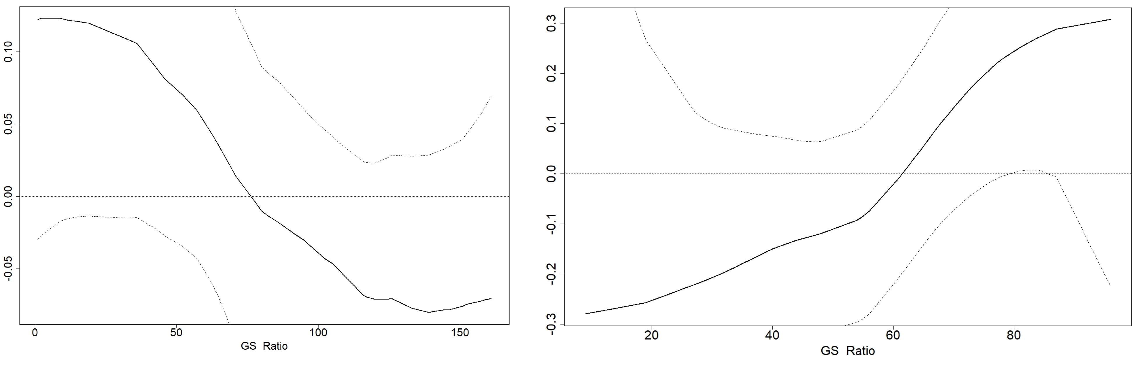
# And plot the non-linear effects (GS ratio and Jandate (when the data were collected)), to see if they have a distinct effect
par(mfrow = c(1,1), mar = c(4,3,1,1))
plot(Mod_Point2$summary.random$GS_Ratio[,1:2],
     type = "l",
     lwd = 2,
     xlab = "GS_Ratio",
     ylab = "",
     cex.axis = 2,
     cex.lab = 2)
for(i in c(4,6))
  lines(Mod_Point2$summary.random$GS_Ratio[,c(1,i)], lty = 2)
abline(h = 0, lty = 3)
The amount of greenspace (GS Ratio) is clearly positively correlated with species richness, but the effect is fairly linear, so we might want to consider fitting it as a linear effect in the next model (we won’t loose much information by doing so).
plot(Mod_Point2$summary.random$JanDate[,1:2],
     type = "l",
     lwd = 2,
     xlab = "Jandate",
     ylab = "",
     cex.axis = 2,
     cex.lab = 2)
for(i in c(4,6))
  lines(Mod_Point2$summary.random$JanDate[,c(1,i)], lty = 2)
abline(h = 0, lty = 3)
Now we can extract some further information about the spatial field.
# Extract the information on the spatial field
Mod_p2.field <- inla.spde2.result(inla = Mod_Point2,
                                  name = "spatial.field2",
                                  spde = spde.pc,
                                  do.transf = T)

inla.emarginal(function(x) x, Mod_p2.field$marginals.kappa[[1]])
inla.hpdmarginal(0.95, Mod_p2.field$marginals.kappa[[1]])

inla.emarginal(function(x) x, Mod_p2.field$marginals.variance.nominal[[1]])
inla.hpdmarginal(0.95, Mod_p2.field$marginals.variance.nominal[[1]])

inla.emarginal(function(x) x, Mod_p2.field$marginals.range.nominal[[1]])
inla.hpdmarginal(0.95, Mod_p2.field$marginals.range.nominal[[1]])
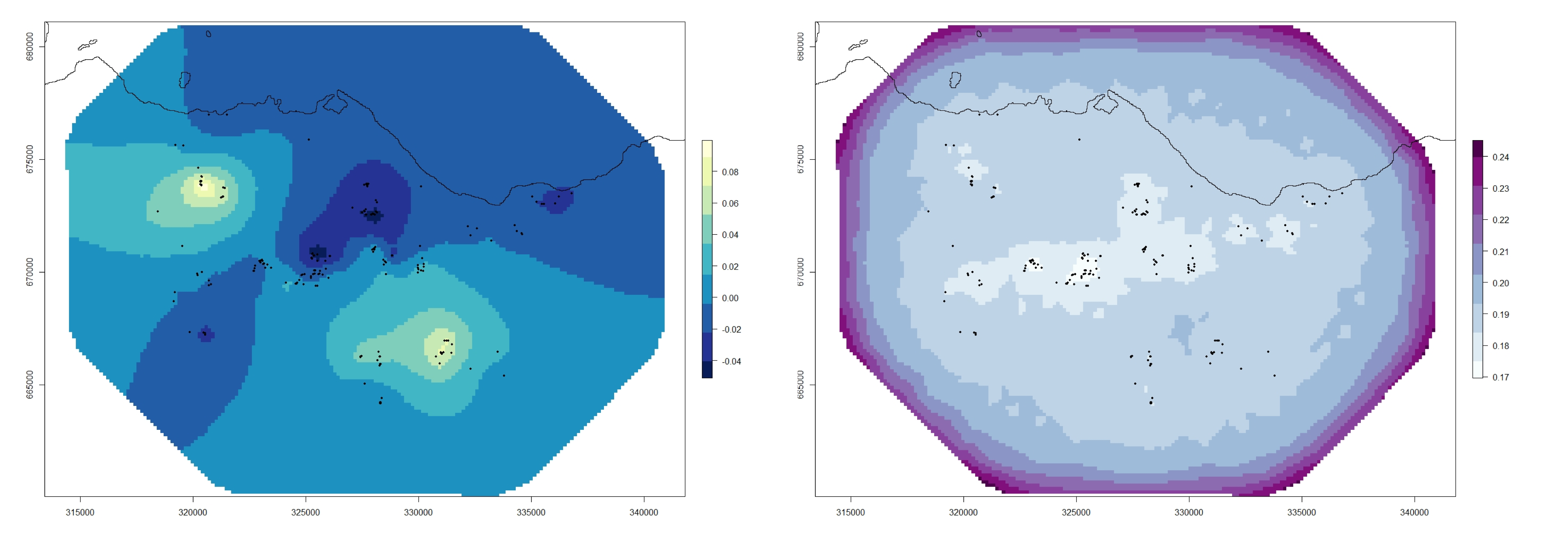
We might also be interested in visualising the Gaussian random field (GRF). As mentioned before, the GRF represents the variation of the response variable in space, once all the covariates in the model are accounted for. It could be seen as “the real distribution of the response variable in space”.
However, this can also reflect the lack of an important covariate in the model, and examining the spatial distribution GRF could reveal which covariates are missing, For example, if elevation is positively correlated with the response variable, but it is not included in the model, we could see a higher posterior mean in areas with higher elevation. A researcher familiar with the terrain would be able to recognise this and improve the model accordingly.
points.em <- Mesh3$loc

stepsize <- 150                           # This is given in coordinates unit (in this case this is straightforward and correspond to 150m)
east.range <- diff(range(points.em[,1]))  # calculate the length of the Easting range
north.range <- diff(range(points.em[,2])) # calculate the length of the Northing range

nxy <- round(c(east.range, north.range)/stepsize)  # Calculate the number of cells in the x and y ranges

# Project the spatial field on the mesh vertices using the inla.mesh.projector() function
projgrid <- inla.mesh.projector(Mesh3,
                                xlim = range(points.em[,1]),
                                ylim = range(points.em[,2]),
                                dims = nxy)
xmean <- inla.mesh.project(projgrid,
                           Mod_Point2$summary.random$spatial.field2$mean)
xsd <- inla.mesh.project(projgrid,
                         Mod_Point2$summary.random$spatial.field2$sd)
We need to create spatial objects for the mean and variance of the GRF.
require(raster)

xmean2 <- t(xmean)
xmean3 <- xmean2[rev(1:length(xmean2[,1])),]
xmean_ras <- raster(xmean3,
                    xmn = range(projgrid$x)[1], xmx = range(projgrid$x)[2],
                    ymn = range(projgrid$y)[1], ymx = range(projgrid$y)[2],
                    crs = CRS("+proj=tmerc +lat_0=49 +lon_0=-2 +k=0.9996012717 +x_0=400000 +y_0=-100000 +ellps=airy +units=m +no_defs"))

xsd2 <- t(xsd)
xsd3 <- xsd2[rev(1:length(xsd2[,1])),]
xsd_ras <- raster(xsd3,
                  xmn = range(projgrid$x)[1], xmx =range(projgrid$x)[2],
                  ymn = range(projgrid$y)[1], ymx =range(projgrid$y)[2],
                  crs = CRS("+proj=tmerc +lat_0=49 +lon_0=-2 +k=0.9996012717 +x_0=400000 +y_0=-100000 +ellps=airy +units=m +no_defs"))
xmean_ras and xsd_ras are raster items and can be exported, stored and manipulated outside R (including in GIS softwares) using the function writeRaster().
Now we can plot the GRF (I used the same colour scheme as the areal data):
par(mfrow = c(1,1), mar = c(2,2, 1,1))
plot(xmean_ras, asp = 1, col = my.palette.post)
points(Fox_Point, pch = 16, cex = 0.5)
plot(Scot_Shape_BNG, add = T)

plot(xsd_ras, asp = 1, col = my.palette.var)
points(Fox_Point, pch = 16, cex = 0.5)
plot(Scot_Shape_BNG, add = T)
Plot spatial predictions and gaussian random field
Finally, I’m going to show how to produce spatial predictions from INLA models. This will involve a bit of manipulation of rasters and matrices (check out the Coding Club tutorial on this subject here if you’d like to learn more about working with rasters in R. Essentially it comes down to creating a spatial grid of coordinates where we do not have values but wish to generate an prediction for the response variable using the model estimations (taking into account the spatial autocorrelation structure of the data).
# The first step is to load the prediction raster file (this one is a ASCII file).
require(raster)
require(rgdal)
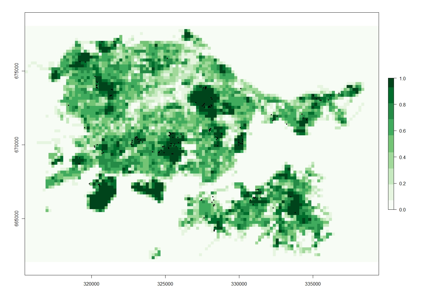
GS_Pred <- raster("GS_Pred/GS_Pred_Raster.txt")
# This is simply a raster map of greeenspace values (precentage of greenspace per raster cell) plotted for the entire Edinburgh area.
require(RColorBrewer)
my.palette_GS <- brewer.pal(n = 9, name = "Greens")
plot(GS_Pred, col = my.palette_GS)
points(Fox_Point, pch = 16, cex = 0.5)
To produce predictions using INLA, we need to generate a dataset (with attached coordinates on the locations we wish to predict to) and attach a series of missing observation to it (coded as NA in R). When the missing observations are in the response variable, INLA automatically computes the predictive distribution of the corresponding linear predictor and fitted values.
Using INLA syntax is possible to generate model preditions by fitting a stack where the response variable is set as NAs, and then join this stack with the estimation stack (which is similar to what we have used so far). Then we can extract the values of the predicted response variable and use the inla.mesh.projector() function to project these values on the mesh vertices (like we have been doing when plotting the GRF earlier on).
To start, we transform the raster values for the amount of green space (GS ratio) into a matrix and then reallocate the coordinates to a matrix of ncol X nrow cells (numbers of columns and rows).
GS_Matrix <- matrix(GS_Pred)

str(GS_Matrix)

y.res <- GS_Pred@nrows
x.res <- GS_Pred@ncols
Next, we need to create a grid of ncol X nrow cells containing the coordinates of the points where we wish to project our model predictions.
Seq.X.grid <- seq(from = GS_Pred@extent@xmin,
                  to = GS_Pred@extent@xmax,
                  length = x.res)

Seq.Y.grid <- seq(from = GS_Pred@extent@ymin,
                  to = GS_Pred@extent@ymax,
                  length = y.res)

pred.grid <- as.matrix(expand.grid(x = Seq.X.grid,
                                   y = Seq.Y.grid))

str(pred.grid)
Now that we the grid with the coordinates of each cell centroid we can procede to make the mesh SPDE and spatial index as usual.
MeshPred <- inla.mesh.2d(Loc, max.edge = c(900, 2000),
                         cutoff = 300)

spde.pred <- inla.spde2.matern(mesh = MeshPred,
                               alpha = 2)

s.index.p <- inla.spde.make.index(name = "sp.field.pred",
                                  n.spde = spde.pred$n.spde)
Since the points where we want to project our predictions are different from the datapoints, we need two different projector matrices. The first one is the standard one we have used so far (A_est), while the second does not contain point locations since we will project the model results directly on the mesh vertices. Similarly, we will need two stacks, one for estimations and one for predictions, joined using the inla.stack() function to form a joined stack.
A_est <- inla.spde.make.A(mesh = MeshPred,
                          loc = Loc)

A_pred <- inla.spde.make.A(mesh = MeshPred)


StackEst <- inla.stack(data = list(y = Point_Data$Spp_Rich),
                       A = list(A_est, 1),
                       effects = list(c(s.index.p, list(Intercept = 1)),
                                      list(GS_Ratio = Point_Data$GS_Ratio2)),
                       tag = "Est")

stackPred <- inla.stack(data = list(y = NA),  # NAs in the response variable
                        A = list(A_pred),
                        effects = list(c(s.index.p, list(Intercept = 1))),
                        tag = "Pred")

StackJoin <- inla.stack(StackEst, stackPred)
Then we can specify the formula and run the model as usual (using the joint stack).
formula_Pred <- y ~ -1 + Intercept +
  f(GS_Ratio, model = "rw2") +
  f(sp.field.pred, model = spde.pred)

Mod_Pred <-  inla(formula_Pred,
                  data = inla.stack.data(StackJoin, spde = spde.pred),
                  family = "poisson",
                  control.predictor = list(A = inla.stack.A(StackJoin),
                                         compute = T))
We need to extract the index of the data from the prediction part of the stack (using the tag “Pred” we assigned to the stack) and use it to select the relevant posterior mean and sd for the predicted response variable. Then we use the inla.mesh.projector() function to calculate the projection from the Mesh to the grid we created (pred.grid).
index.pred <- inla.stack.index(StackJoin, "Pred")$data

post.mean.pred <- Mod_Pred$summary.linear.predictor[index.pred, "mean"]
post.sd.pred <- Mod_Pred$summary.linear.predictor[index.pred, "sd"]

proj.grid <- inla.mesh.projector(MeshPred,
                                 xlim = range(pred.grid[,1]),
                                 ylim = range(pred.grid[,2]),
                                 dims = c(x.res, y.res))
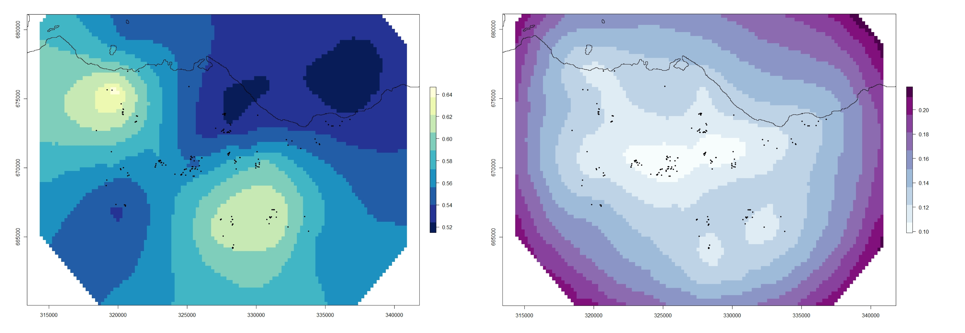
Finally, we project the values we extracted from the model on the lattice we have created and transform the projected predictions to a raster object as we did before with the GRF and plot them in a similar fashion (we do this for both the mean and standard deviation).
post.mean.pred.grid <- inla.mesh.project(proj.grid, post.mean.pred)
post.sd.pred.grid <- inla.mesh.project(proj.grid, post.sd.pred)

predmean <- t(post.mean.pred.grid)
predmean2 <- predmean[rev(1:length(predmean[,1])),]
predmean_ras <- raster(predmean2,
                      xmn = range(projgrid$x)[1], xmx = range(projgrid$x)[2],
                      ymn = range(projgrid$y)[1], ymx = range(projgrid$y)[2],
                      crs = CRS("+proj=tmerc +lat_0=49 +lon_0=-2 +k=0.9996012717 +x_0=400000 +y_0=-100000 +ellps=airy +units=m +no_defs"))

predsd <- t(post.sd.pred.grid)
predsd2 <- predsd[rev(1:length(predsd[,1])),]
predsd_ras <- raster(predsd2,
                       xmn = range(projgrid$x)[1], xmx = range(projgrid$x)[2],
                       ymn = range(projgrid$y)[1], ymx = range(projgrid$y)[2],
                       crs = CRS("+proj=tmerc +lat_0=49 +lon_0=-2 +k=0.9996012717 +x_0=400000 +y_0=-100000 +ellps=airy +units=m +no_defs"))

# plot the model predictions for mean
par(mfrow = c(1,1), mar = c(2,2, 1,1))
plot(predmean_ras, asp = 1, col = my.palette.post)
points(Fox_Point, pch = 16, cex = 0.5)
plot(Scot_Shape_BNG, add = T)

# plot the model predictions for sd
par(mfrow = c(1,1), mar = c(2,2, 1,1))
plot(predsd_ras, asp = 1, col = my.palette.var)
points(Fox_Point, pch = 16, cex = 0.5)
plot(Scot_Shape_BNG, add = T)
In the interest of keeping this tutorial short(ish), I have only presented an example of producing model predictions at unsampled locations. But keep in mind that producing predictions for model validation is relatively straightforward (e.g., when you want to check how the real values and the model predictions compare, and you should be able to do it using the code I presented here as a template). Feel free to have a go if you’d like a challenge!
You just need to split the dataset in two (one part used for estimation, the other for validation) and assign NAs to the response variable of the validation subset (while retaining coordinates and the rest of the covariate), then prepare a separate validation projection matrix (A_Val) and a validation stack, similarly to what we have done here. Finally, when you run the model you can access the predicted values for the validation data by using the inla.stack.index() function and use it to evaluate the predictive power of your model.
Final Remarks
You made it through the tutorial, well done!!!
After this you should be able to fit basic spatial models of area and marked point data, extract results and make predictions. Spatial modelling is becoming increasingly popular and being able to account for autocorrelation in your modelling is a great skill to have.
There is probably still much more you want to know. The good news is that INLA is extremely customisable and you can modify it to do almost anything you need.
The R-INLA project is under active development, and the INLA project website is a great place to go to find materials (including tutorials, examples with explanations and code from published articles) and help: the R-INLA discussion group is very active and it is a great place to go if you get stuck.
There are also a number of books and tutorials (I have mentioned a few but so many more are available), most of which are freely available to download (including the code), or available in the library if you’re a student.
Stay up to date and learn about our newest resources by following us on Twitter!
Contact us with any questions on ourcodingclub@gmail.com
- Analysing and visualising population trends and spatial mapping
- Analysing and visualising population trends and spatial mapping