Tutorial Aims:
- Get acquainted with data clustering
- Learn about different distance metrics
- Learn about different linkage methods
- Turn groups into a grouping variable
- Map cluster groups in geographic space
To get all you need for this session, go to the repository for this tutorial, fork it to your own Github account, clone the repository on your computer and start a version-controlled project in RStudio. For more details on how to do this, please check out our Intro to Github for version control tutorial. Alternatively you can download the repo as a zip file.
1. Get acquainted with data clustering
Hierarchical data clustering allows you to explore your data and look for discontinuities (e.g. gaps in your data), gradients and meaningful ecological units (e.g. groups or subgroups of species). It is a great way to start looking for patterns in ecological data (e.g. abundance, frequency, occurrence), and is one of the most used analytical methods in ecology. Your research questions are the limit. Hierarchical clustering offers insight into how your biodiversity data are organized and can help you to disentangle different patterns and the scales at which they can be observed. For example, you could use data clustering to understand algae distribution along a ocean depth gradient, or look at the distribution of bats along an elevation gradient, or study how fish communities are distributed along water basins and see if rapid streams and waterfalls are limiting their dispersal, or even determine which are the main biogeographic realms in the world.
Let’s imagine the following: you are an ecologist working on tropical forests in the Neotropics and you want to understand how these forests, composed of different species of tree, are related to one another. You could use data clustering to split them into ecologically meaningful sub-groups that can then be used as a grouping variable (a categorical variable) in future analyses. You might be interested in questions such as: How many ecologically meaningful floristic units are present in the Neotropics? Which ones are more similar to each other? How many species do they share? How are these units distributed in geographic space? Does each unit occupy a certain portion of the geographic space, or is the spatial distribution of units mixed?
You can then build your next set of research questions based on the answers you got from the data clustering. What are the environmental drivers of the patterns in my data? Is climate one of these drivers? How will these tree groups respond to climate change? Are these floristic units related to climate? In such a big region (the Neotropics), are there biogeographic and environmental barriers separating these units? Do you get clear splits from one group to another or do you get a gradient of floristic turnover across the border of two of these floristic units?
To answer these questions, you can construct a dataset which consists of tree species occurrence records for a multitude of sites in the Neotropics and perform a series of hierarchical clustering analyses.
Hierarchical agglomerative data clustering
Hierarchical agglomerative data clustering is one part of the broader category of “data clustering”.
Data clustering methods:
- Sequential and simultaneous - refers to how the clustering is conducted. If it’s through an algorithm that is repeated till all data have been clustered, it’s sequential. If the algorithm clusters all your data together at the same time, it’s simultaneous.
- Agglomerative and divisive - refers to how your data are being grouped. Agglomerative is a bottom up approach, meaning that the clustering will begin by putting similar observations together, gradually forming subgroups till all your observations are included. Divisive is the exact opposite, your set of observations will be considered as whole group and the algorithm will divide your data into progressively smaller chunks till each observation forms a sub-group on its own.
- Monothetic and polythetic - refers to the amount of descriptors being employed to cluster your data into subgroups. If it uses just one descriptor on every step, it’s monothetic; if it uses more than one, it’s polythetic.
- Hierarchical and non-hierarchical - hierarchical means that your groups will be organized in ranks according to how similar they are. You’ll have sub-groups forming larger groups till all your observations are included in your cluster. Non-hierarchical clustering methods do not include that option.
In sum, hierarchical agglomerative clustering methods group your observations in increasingly large subgroups till all observations are included. The subgroups formed by the clustering are ordered in ranks according to their level of similarity.
Create a new R script file and start working your way through the tutorial
We find having the tutorial on half of your screen, and RStudio on the other half, useful for following along and seeing what the results of each code chunk are. For today’s session, we’ll be working with four different packages. Please install them and load their libraries:
install.packages("recluster")
install.packages("phytools")
install.packages("maps")
install.packages("vegan")

# Loading libraries
library(recluster)
library(phytools)
library(maps)
library(stats)
library(cluster)
As you might have realised by now, I work on tropical trees and forests in the Neotropics, and today I have decided to give you a quick tour through some of the amazing forests and floristic formations we have there. Today’s destination is Bolivia, a large country in tropical South America with just about ten million people living in it. Most of these people live in four gigantic cities: La Paz, Sucre, Cochabamba and Santa Cruz de La Sierra. As a result, most of Bolivia’s diversity is located away from human settlements and is, therefore, relatively protected from human impact. Biogeographically, Bolivia is where all the main Tropical South American biomes converge. This makes Bolivia one of the most interesting and exciting places to study (and visit) in South America.
The data we’ll be using today come from a dataset called NeoTropTree which was developed by Professor Ary Oliveira-Filho (Federal University of Minas Gerais - Brazil). NeoTropTree is a large database containing records on forest tree species composition, gathered by reviewing the literature (published and unpublished - e.g. masters dissertations and PhD theses), compiling species check-lists, and studying herbarium records. Each site within the database has been assigned to a specific vegetation type (an ecologically meaningful unit). NeoTropTree is a very comprehensive and well kept dataset, which makes it very valuable and reliable when doing science. Professor Oliveira-Filho has kindly agreed to us using a tiny portion of it for this tutorial.
# Loading the dataframes we'll be working with:
# First load the data-frame containing all species for which NeoTropTree has at least one record in Bolivia.
spp <- read.csv("spp_bol.csv", sep=",", head=TRUE)
head(spp)  # View the first few columns
dim(spp)  # How many rows and columns are there?
Each species has a SppID number and a code, which is in the Species.code column. These two columns will be of major importance to us later on. There are 3369 tree species registered for Bolivia in NeoTropTree.
# Load the dataframe containing all sites NeoTropTree has in Bolivia.
sites <- read_csv("sites_bolivia.csv", sep=",", head=TRUE)
head(sites)
dim(sites)
Each site has an AreaID, an Area Code, information on locality, vegetation type, geographic coordinates and elevation. You can also see that the sites are classified in Phytogeographic Domains (Domain). This is important because the AreaCode column, to which we’ll be referring very often, is based on these domains - the first three letters of an area code correspond to the Domain on which the site is located. Sites beginning with Amz, are a part of the Amazon Domain; And = Andes; Cer = Cerrado (South American savannas); Cha = Chaco woodlands (mainly subtropical, shrubby, mostly deciduous and dry floristic formation). Pay attention to this, as this will be very important when looking for sub-groups in our dataset.
Now it’s time for us to load the correspondence matrix, a matrix indicating what species are present on which site, information that is vital to us in order to make a presence and abscence matrix.
# Load the sppxarea matrix
sppxsites <- read.csv("sppxsites_bol.csv", sep=",", head=TRUE)
head(sppxsites)
dim(sppxsites)
Please note that you only have two columns in here - SppID and AreaID.The number of rows is the number of occurrence records in our dataset - 42015.
Making a presence/absence matrix through a loop
How does the chosen clustering method know which observations are more similar to one another than others? Simple. You will provide it with a pairwise distance matrix. This is a quadratic (number of rows is equal to the number of columns) matrix containing the distance values taken for each pair of sites in the dataset. There are different ways of calculating these pairwise distances and the most suitable method for you will largely depend on the kind of data you are working with.
Right now, what we need to do is use the data frames we have and create a presence and absence matrix with sites in the rows and species in the columns. As it is standard, 1 = species present in a site and 0 = the species absent in a site. No matter what distance metric you use, the pairwise distance matrix that will be used when clustering your data will always be constructed based on this table. Of course, if you have species abundance, than you’ll be working with an abundance matrix.
The way we are going to build such matrix is through a loop function. Loop functions are extremely useful used in many programming languages. If you want to learn more about them, you can check our tutorial on how to use loops.
# Making the species by site matrix (presence and abscence). We'll call it `commat`.

sites_sub <- unique(sppxsites$AreaID)  # Making a vector with sites in our dataset
spp_sub <- unique(sppxsites$SppID)  # Making a vector with species in our dataset

# First we'll create an empty matrix with our sites in the rows and our species in the columns. The loop function will place a `1` on a given cell when the species is present in an area and will fill out the remaining cells with a `0`.

spp_commat <- matrix(0, length(sites_sub), length(spp_sub))
for (i in 1:nrow(spp_commat)){
  temp_sites <- sppxsites[which(sppxsites$AreaID == sites_sub[i]),]
  spp_commat[i, which(spp_sub%in%temp_sites$SppID)] <- 1
  print(i)
}

# Now let's name our rows and columns with the codes for the sites and the codes for the species.
rownames(spp_commat) <- as.character(sites$AreaCode[match(sites_sub, sites$AreaID)])
colnames(spp_commat) <- as.character(spp$Species.code[match(spp_sub, spp$SppID)])
dim(spp_commat)

# Check if the loop function worked alright and did its job
spp_commat[1:6,1:6]
When working with large presence/absence datasets, it is good practice to remove “uniques”. “Uniques” are species that only have one recorded presence in only one observation/sample. The reason behind this is that such species will only bring noise (somewhat random, hard to explain variation) to the analysis and will only blur the patterns we get. Later on, for the sake of practice, we’ll compare the results we’ll get with the full presence and absence matrix with the results we’ll get with the same matrix without any “Uniques”.
spp_commat_trim <- spp_commat[,which(!colSums(spp_commat) == 1)]
dim(spp_commat_trim)

# We removed 275 species from our dataset. We'll check if this makes much of a difference later on.
2. Distance Metrics
To learn which distance measures are available to us, check out:
help("vegdist")
help("recluster.dist")
I know, these are scary, complicated and lengthy lists filled with things that you may not understand that well (or at all!). Don’t worry though, the most used distance metrics in hierarchical data clustering are the Euclidean distance metric, the Jaccard index, Sorensen distance, Simpson distance metric (pay attention: this is not the Simpson diversity index) and Bray-Curtis.
You have to be careful when using Euclidean and Sorensen distances, as they tend to be heavily influenced by big differences in species frequencies (our case), a lot of absences in the matrix (our case), and a great amount of observations (surprise, surprise, our case). Do avoid them in case your dataset meets any of these conditions. On such occasions, use Simpson instead, as it is a distance metric that deals very well with these issues and is becoming increasingly common in ecology. Euclidean is good for continuous data in general, Sorensen as well. You can use adapted Jaccard indices for abundance and occurrence data. Bray-curtis and Morisita-Horn are used for abundance data. And similar to Jaccard, there are different Simpson equations to estimate distance based on abundance or occurrence data.
This can be a bit of a stretch, but it is worthwhile mentioning that, in most cases, you’ll be working with beta diversity when calculating these distance matrices. Beta diversity can be decomposed into two components: turnover and nested-ness.
Turnover refers to when you have species replacing each other over an environmental gradient or geographic space. Nestedness refers to when a site/sample is occupied by a fraction, a subset, of the surrounding species pool, not by new species (nestedness is commonly associated with environmental filtering). Depending on the patterns you want to look at and how big your dataset is in terms of scale, these fractions must be taken into account. Jaccard distance is defined as turnover + nestedness = 1, Simpson focus on species turnover only, so it is great for biogeographic analysis.
The Simpson distance metric (not Simpson’s diversity index) is becoming increasingly common in ecology for the reasons described above. Since our dataset is big, not very well balanced and filled with absences, we’ll be using it in our analyses today and will not pay attention to the other distance metrics. Besides, it is wise for us to focus only on species turnover, since we are working on such a broad geographic scale.
# Picking a metric is difficult, but calculating it is actually simple. Simply use the recluster.dist command or the vegdist command in order to estimate such distances.
simpson_dist <- recluster.dist(spp_commat_trim, dist="simpson")
jaccard_dist <- recluster.dist(spp_commat_trim, dist="jaccard")
sorensen_dist <- recluster.dist(spp_commat_trim, dist="sorensen")
euclidian_dist <- vegdist(spp_commat_trim, method="euclidean")
Distance metrics are a very broad topic that deserves a tutorial on it’s own and we only covered a tiny portion of it. You should definitely explore this topic more when clustering your own data. There is one more thing we need to know before we start clustering - linkage-methods.
3. Linkage Methods
The linkage method is the criterion that will determine how your observations will be grouped together. Here, we’ll discuss the most commonly used linkage methods in ecology:
- Single-linkage method (single dendogram)
- Single-linkage method (concensus dendogram)
- Complete-linkage method
- Clustering using Ward’s minimum variance
- Average linkage
Run this code to check out the linkage methods that are available to us:
help(hclust)
The function we’ll be using today recluster.cons uses the Simpson’s distance metric by default and that is what we will be using in this tutorial. The recluster.dist function makes the pairwise distance table for you, all you have to do is select the distance metric you want.
Single-linkage method (single dendogram)
This method is the simplest of them all. It links observations according to the shortest pairwise distance in your distance matrix. A given observation will be linked to a group if the distance between this site and any other element within that group is the shortest one available at that step. This is not a very strict criterion and can lead to weird group formations if your dataset is very big and you have many equally similar observations.
bol_singlelink <- recluster.cons(spp_commat_trim, tr = 1, p = 0.5, dist = "simpson", method = "single")
bol_singlelink_tmp <- bol_singlelink$cons  # Selecting the consensus tree (we'll discuss it later)
plot(bol_singlelink_tmp, direction = "downwards", cex = 0.5)  # You can change the "direction" argument to your liking.

# the write.tree function will let you save your cluster in TRE format so you can open it with Figtree and visualise it better.
write.tree(bol_singlelink_tmp, "bol_singlelink_tmp.tre")
Let’s open this file in Figtree and see how we can use this software to our advantage. You can quickly download Figtree for your operating system here and install it on your computer. Figtree was originally designed to look at phylogenies, but we can use it to visualise dendograms (the outputs of our data clustering are called dendograms). You simply click on the document you want to open and select Figtree to open it. You can select branches and colour them to your liking with the Colour button. You can also zoom in with the Zoom button, allowing you to read the names on the tips of your dendogram and visualize your groups.
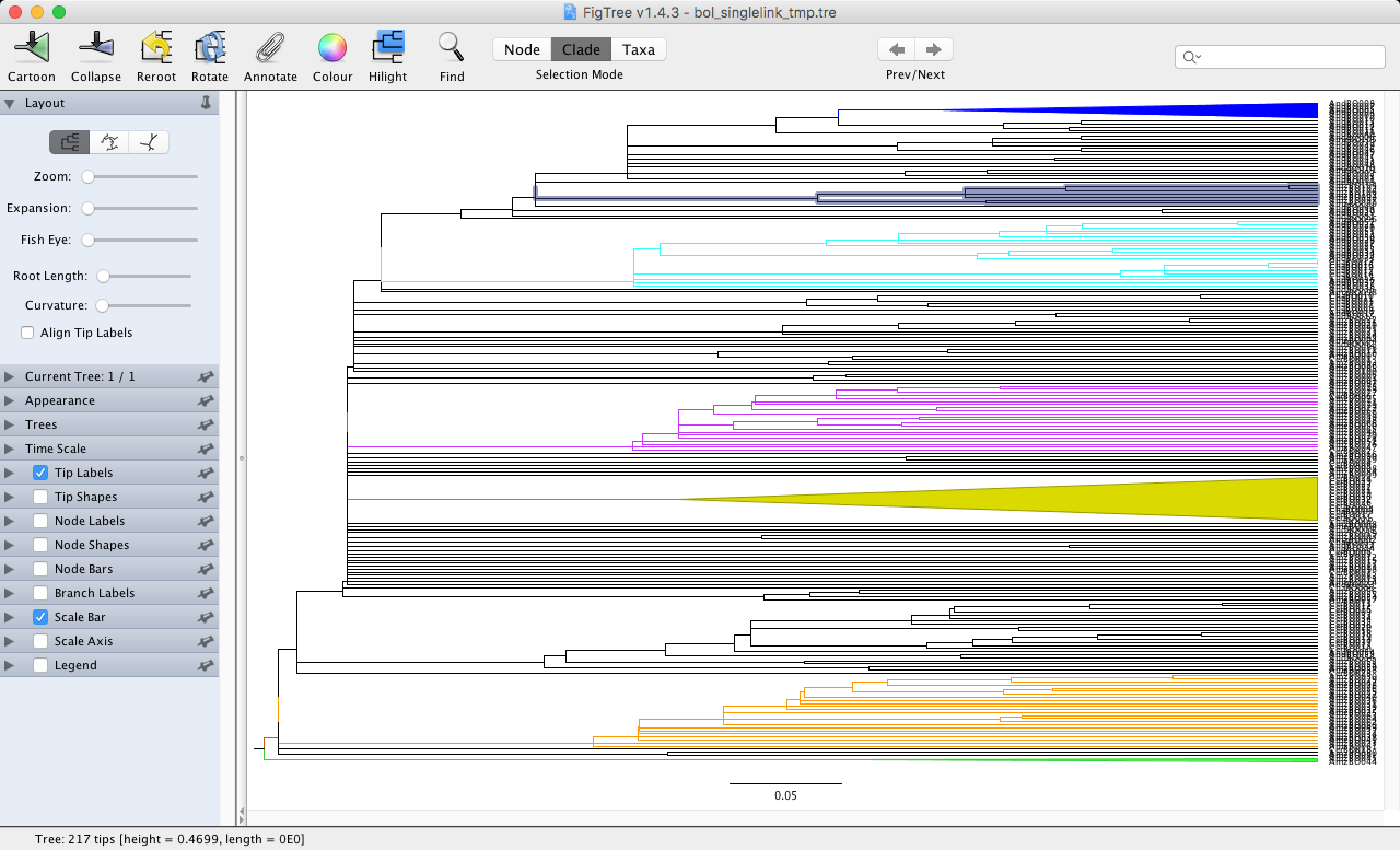
As you can see in the dendogram, we do not have any clearly defined groups. This is to be expected when using the single-linkage method, which is good for examining gradients in the dataset. You can still see some small groups scattered across the dendogram that are mainly formed by Amazonic (starting with Amz) and Andean (starting with And) sites.
Now that we have made our first cluster (congratulations!), there is something else you need to know. We are clustering data from a big dataset by using a distance matrix that most likely has many observations that are equally similar to one another. This means that these sites/samples can be clustered together in different ways and each way would be equally correct. How can we deal with this problem?
The answer is simple: we will build a solution which reflects the groups we encountered across different clusters made with the same distance matrix and the same linkage method. In other words, the solution will be made through a consensus. We will establish a criterion of inclusion that will indicate the number of times a certain subgroup/branch was recovered in a pool of equally valid solutions (dendograms) to our clustering problem. This is determined through the p argument. p can be any number ranging from 0.5 to 1 (recovered in 50% of the dendograms to recovered in 100% of the dendograms). Smaller numbers will give you a better chance of recovering sub-groups in your consensus dendogram. Numbers close to 100% will diminish that chance. The number you assign to the p argument largely depends on your research questions and on how stable you want your groups to be. The size of our solutions pool (equally possible and valid dendograms) is determined by the tr argument, the standard number to use here is 100.
Now, let’s see if we can get a better solution when using different, equally valid, dendograms to come up with a solution to our clustering problem.
Single-linkage method (concensus dendogram)
bol_singlelink <- recluster.cons(spp_commat_trim, tr = 100, p = 0.5, method = "single")
bol_singlelink_cons <- bol_singlelink$cons
write.tree(bol_singlelink_cons, "bol_singlelink_cons.tre")
plot(bol_singlelink_cons, direction = "downwards", cex = 0.5)
Apart from a few sites changing their positions, the dendogram doesn’t look that different. This is largely because we have a lot of individual sites being treated as single groups. The order in which these sites are presented is not important, because the relationship between them is the same (they come up from the same node). There aren’t many differences in the solution because there is nothing much to vary in here, most groups are coming out of the same node.
Now we will move on to the other methods and we will always work with the solution reached through the application of the consensus criterion (p=0.5)
Complete-linkage method
Using the complete-linkage method, an observation is only allowed to be linked to a subgroup when it is more related to it than to the most distant pair of observations in that group. By doing so, when a observation is linked to a subgroup, you can assume that it is related to all observations in that group.
bol_completelink <- recluster.cons(spp_commat_trim, tr = 100, p = 0.5, method = "complete")
bol_completelink_cons <- bol_completelink$cons
write.tree(bol_completelink_cons, "bol_completelink_cons.tre")
plot(bol_completelink_cons, direction = "downwards", cex = 0.5)
This is a great example of how important selecting a linkage method is! Look how well defined the groups are now, even though there are no clear relationships between the subgroups we’ve got (they all come out of the same node). Since the linkage criterion is more strict, the groups are better defined. You can open the file you’ve just created in Figtree and explore the subgroups.
The complete linkage method allows you to highlight discontinuities in your dataset, i.e. find out about potential gaps in your data. However, be advised that it is important for these groups to be ecologically meaningful and that is up to you to decide what that means. In here, you were given the phytogeographic domain in which these sites are located and how each site was classified according to its vegetation structure and other characteristics. You can use that in order to verify if these groups make sense from an ecological perspective.
Clustering using Ward’s minimum variance
This is a special kind of linkage method designed to form groups in a way that minimises the within group sum of squares (within total sum of squares expresses the amount of vegetation in each subgroup). This method is usually advisable when the groups obtained through data clustering will be used as categorical variables in subsequent analyses, such as ANOVAs and MANOVAs.
bol_ward <- recluster.cons(spp_commat_trim, tr = 100, p = 0.5, method = "ward.D")
bol_ward_cons <- bol_ward$cons
plot(bol_ward_cons, direction = "downwards", cex = 0.5)
write.tree(bol_ward_cons, "bol_ward_cons.tre")
This dendogram’s topology (‘dendogram topology’ refers the branching pattern relationship among individuals) is different from the other two dendograms we produced before. How many main groups can you see in here? Considering the phytogeographic domains in which these sites are located, are these groups ecologically meaningful? Why don’t you open the cluster you created with the complete linkage method and compare it with this one? How different are they? Which one would you use in order to perform further analysis?
Average linkage method (UPGMA) and an observation on “uniques” and potential biases in the dendograms
Remember that I said we would investigate if there are any differences between the results you obtain with the complete presence/absence matrix and the matrix without any “uniques”? We are going to do it now. Will removing “uniques” improve the resolution within your dendograms or not? We’ll discover as soon as we learn more about the Average linkage method.
UPGMA stands for unweigthed Pair-Group Method Using Arithmetic Averages. Big name, I know. However, the name pretty much says how this linkage-method will link our observations: it will link our sites/samples by considering their distance to a subgroup’s arithmetic average (calculated using the pairwise distances). This is a very sensible linkage-method that usually tends to form ecologically meaningful groups and it is one of the most used hierarchical linkage methods in ecology, especially in biogeography. This is why the rest of our analyses will focus on this particular linkage method.
# Full species presence/abscence matrix

bol_upgma <- recluster.cons(spp_commat, tr=100, p=0.5, method = "average")
bol_upgma_cons <- bol_upgma$cons
write.tree(bol_upgma_cons, "bol_upgma_cons.tre")
plot(bol_upgma_cons, direction = "downwards", cex=0.5)

# Trimmed species presence/abscence matrix

bol_upgma_trim <- recluster.cons(spp_commat_trim, tr=100, p=0.5, method = "average")
bol_upgma_trim_cons <- bol_upgma$cons
write.tree(bol_upgma_trim_cons, "bol_upgma_cons_trim.tre")
plot(bol_upgma_trim_cons, direction = "downwards", cex=0.5)
Removing “uniques” in this particular analysis didn’t change our dendogram. This is a good thing: it means that we can keep work with the most complete form of the dataset without having to worry about bias. However, depending on the analysis you’ll do afterwards, it is advisable to remove these species anyway, just to be on the safe side.
Bootstrap and support values for subgroups
Bootstrapping is one of the main ways of calculating support values for the subgroups we have got in our dendogram. It is usually used to test significance through randomisation procedures. However, since hierarchical clustering analysis do not work with significance, here bootstrapping assesses whether you’ll get the same subgroups in a dendogram even if you resample the species occurring in each site (with replacement - meaning you can repeat species and even not include some species at all. Bootstrap values range from 0 to 100 and express the proportion of times a certain subgroup was recovered during the resampling. The bigger the number, the stronger the subgroup.
However, bootstrap values tend to decrease when you have matrices with an unequal data distribution (a lot of zeroes). In our case, we have many sites and groups with low species richness. During the resampling, the calculation will end up removing species that are important to define groups, bringing the support values down, since the same groups will not be recovered. So don’t get frustrated by the low values we get, as bootstrapping is not useful in our case. Nevertheless, bootstrap values tend to be reliable when you have equally distributed data.
The boot argument tells the function how many randomizations you want to make before calculating the bootstrap values. The bigger the number, the longer it will take for your computer to run it. The standard number is 1000, but that takes at least three hours till you to get results. So we are going to set it to 10 instead.
bol_upgma_trim_boot <- recluster.boot(bol_upgma_trim_cons, spp_commat_trim, tr = 100, p = 0.5, method = "average", boot = 10, level = 1)
recluster.plot(bol_upgma_cons, bol_upgma_trim_boot, direction = "downwards")
There are some high values for a few of the groups in here, but if you set the boot value to a higher number (100 - 1000), the support values you found will go down.
4. Creating a grouping variable
It would be interesting to visualise the spatial distribution of the groups you found in your cluster. To do that, you need to create a vector linking the plant observations to the cluster they belong to. We have to make R acknowledge the existence of polytomies in our dendograms. Polytomies are the nodes that lead to more than two nodes/tips and/or groups (pretty much what we got when using the simple linkage method, remember?).
If you type the name of your consensus tree on your console, you get a quick summary of your cluster (it says that it is a phylogenetic tree, but it’s a dendogram), and how many tips (terminal branches) and nodes (ramifications) it has.
bol_upgma_trim_cons
A dendogram with no polytomies will have x tips and x-1 internal nodes. However, all dendograms we have produced so far will have this number, because R does not automatically recognize polytomies. Let’s use the di2multi function from the phytools package and identify these politomies.
bol_upgma_cons
bol_upgma_cons_nodi <- di2multi(bol_upgma_cons)
bol_upgma_cons_nodi
This cluster in particular has just four politomies, but others might have more than that. Always use this command, even if you are pretty sure you don’t have any polytomies. Depending on how big your dendogram is, it can be hard to assess presence or absence of polytomies visually. Let’s take a look at what this function will do to a dendogram with a lot of polytomies in it.
bol_singlelink_cons
bol_singlelink_cons_nodi <- di2multi(bol_upgma_trim_cons)
bol_singlelink_cons_nodi

# We went from 216 nodes to 127 nodes in here. Impressive!
This step is important because we want to create a vector with our cluster groups and if the presence of polytomies is not acknowledged now, we are going to have a hard time in the near future. Let’s create the vector with the politomy-free dendogram. We will call it cluster memberships. The vector can also be used to do further analysis where the cluster groups are a categorical (grouping) variable, for example mapping our sites on a map of Bolivia, or running PCAs, NMDSs, PCoAs, and more.
We will now determine the node that links together all sites in one of our subgroups (this will be done through the findMRCA function in the phytools package) and then we’ll get all tips and internal nodes connected to the node we’ve selected. After that, we’ll remove the internal nodes and get just the dendogram tips in our group of sites.
When doing this, it is standard procedure to cut a dendogram into subgroups at the same level and not at different levels (you are working with ranks, remember). Imagine yourself placing a ruler horizontally across your dendogram on your computer screen. This is how you cut your cluster into subgroups. As for the level where you want to make the cut, it’s largely up to you, but keep in mind that you want to create units that will summarize the variation in your data. Most ecologists will aim at cutting their dendograms in a way that will produce the smallest possible number of ecologically meaningful subgroups. Of course, if you must, you can cut your cluster at different rank levels, it depends on the units you want to create. But remember this: cutting groups at different rank levels might make your subsequent analyses harder to interpret.
We will cut our dendogram bol_singlelink_cons at one of the deepest levels possible (towards the base of the dendogram). That will give us four subgroups to work with. By looking at the phytogeographic domain, it seems that we’ve got a group which is mainly Amazonic (group1), a small group which is partially amazonic and savannic (group2), a group which is composed mainly of savannas (group3) and a group which seems to be Andean (group 4).
5. Plotting our cluster groups on a map
On the first line (the one with the findMRCA function), you’ll have to cite the names of the tips at the “beginning” and “end” of your subgroups. You’ll notice that I’ve written some site codes in here. These are the names I’ve got on my cluster, but this will probably change from one computer to the other, so you’ll need to open the bol_singlelink_cons object on figtree and look for the necessary tip names yourself. My guess is that most of you will get the same tips I have placed here, but don’t worry if your dendogram looks different from the one in here. Simply change the names on the code and you’ll be fine.
#Group 1 tips
group1_node <- findMRCA(bol_upgma_cons_nodi, c("AmzBO066", "AmzBO033"))  # Get the node that connects all observations between the interval you set (in this cases, observations between"AmzBO066" and "AmzBO033").
group1_tips <- getDescendants(bol_upgma_cons_nodi, group1_node)  # Get all nodes and tips linked to the node you have determined above.
group1_tips <- na.omit(bol_upgma_cons_nodi$tip.label[group1_tips])  # Remove the nodes (NAs) and return just the tips to you.
length(group1_tips)  # Count the number of tips you've got for each group. This will be useful to check if the code worked well.
# 90 tips

#Group 2 tips
group2_node <- findMRCA(bol_upgma_cons_nodi, c("CerBO012", "AmzBO044"))
group2_tips <- getDescendants(bol_upgma_cons_nodi, group2_node)
group2_tips <- na.omit(bol_upgma_cons_nodi$tip.label[group2_tips])
length(group2_tips)
# 28 tips

#Group 3 tips
group3_node <- findMRCA(bol_upgma_cons_nodi, c("AndBO034", "CerBO018"))
group3_tips <- getDescendants(bol_upgma_cons_nodi, group3_node)
group3_tips <- na.omit(bol_upgma_cons_nodi$tip.label[group3_tips])
length(group3_tips)
# 52 tips

# Group 4 tips
group4_node <- findMRCA(bol_upgma_cons_nodi, c("AndBO046", "AndBO018"))
group4_tips <- getDescendants(bol_upgma_cons_nodi, group4_node)
group4_tips <- na.omit(bol_upgma_cons_nodi$tip.label[group4_tips])
length(group4_tips)
# 47 tips
Now that we have the tips, we need to check if any tip was left behind. This is done by simply summing the amount of tips we’ve got for each group and seeing if we get all 217 tips that we have in our dendogram.
90+28+52+47
# There you go. Everyone is here.
Let’s make the vector linking the plant observations to the cluster they belong to, and bind it with our sites data frame.
all_tips <- c(group1_tips, group2_tips, group3_tips, group4_tips) #First we put all tips together
cluster_membership <- vector("character",length(all_tips)) #Then we create a vector as long as the object all_tips
cluster_membership[which(all_tips%in% group1_tips)] <- "Group 1" #Then we assign each set of tips to a subgroup
cluster_membership[which(all_tips%in% group2_tips)] <- "Group 2"
cluster_membership[which(all_tips%in% group3_tips)] <- "Group 3"
cluster_membership[which(all_tips%in% group4_tips)] <- "Group 4"
length(cluster_membership)
class(cluster_membership)
We need to match the sites’ order in the cluster_membership object with the order we have on the sites data frame, so we can correctly add cluster_membership as a column in sites.
cluster_membership <- cluster_membership[match(sites$AreaCode, all_tips)]
#Binding "cluster_membership" to "sites"

sites_membership <- cbind(sites, cluster_membership)
unique(sites_membership$cluster_membership)  # Checking if all groups are in here
dim(sites_membership)
head(sites_membership)  # The cluster-membership column is now added.
Now we are going to map these sites in geographic space. This is a great way to check if these units make sense ecologically and geographically. What should we expect here? Will these groups be separate or inter-dispersed? What are the possible factors behind the patterns we are about to observe? Could it possibly be climate? Are there any biogeographic or environmental barriers setting these groups apart?
Clustering methods do not provide us with direct answers to these questions, but it is a great way for you to start exploring what the possible answers might be.
Visualising the results of our clustering on a map
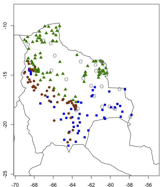
We can now create our map using the following code:
map(xlim = c(-70, -55), ylim = c(-25, -8))  # setting the lat and long limits on our map
map.axes()
# Group 1
points(sites_membership$Long10[which(sites_membership$cluster_membership == "Group 1")]  # Colour-coding by group.
       ,sites_membership$Lat10[which(sites_membership$cluster_membership == "Group 1")], pch = 24, col = rgb
       (t(col2rgb("chartreuse4"))/255, alpha=1), bg = rgb(t(col2rgb("chartreuse4"))/255))

#Group 2
points(sites_membership$Long10[which(sites_membership$cluster_membership == "Group 2")]
       ,sites_membership$Lat10[which(sites_membership$cluster_membership == "Group 2")], pch = "O", col = rgb
       (t(col2rgb("gray53"))/255,alpha=1), bg = rgb(t(col2rgb("gray53"))/255, alpha=1))

#Group 3
points(sites_membership$Long10[which(sites_membership$cluster_membership == "Group 3")]
       ,sites_membership$Lat10[which(sites_membership$cluster_membership == "Group 3")], pch = 15, col = rgb
       (t(col2rgb("blue"))/255,alpha=1), bg = rgb(t(col2rgb("blue"))/255, alpha = 1))

#Group 4
points(sites_membership$Long10[which(sites_membership$cluster_membership == "Group 4")]
       ,sites_membership$Lat10[which(sites_membership$cluster_membership == "Group 4")], pch = 19, col = rgb
       (t(col2rgb("saddlebrown"))/255,alpha = 1), bg = rgb(t(col2rgb("saddlebrown"))/255))
Which creates this map:
Congratulations on completing the tutorial!!! I know the explanations were a bit long, but we needed to cover the theory before doing the clustering. Keen to practice your data clustering and spatial visualisation skills? Check out our challenges below!
Challenge number 1
We mapped our sites using the maps package associated with R’s basic plot function and its arguments.
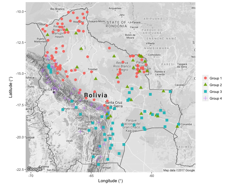
Try recreating the above map using the ggmap package, which offers more choices of map types and in general can make very pretty maps.
In previous versions of this workshop, we used the ggmap package in our tutorial on spatial visualisation, but this package has become difficult to use, especially since Google now requires a non-free API key to download their map tiles. There are lots of other resources online for ggmap and I’d still recommend having a look if you have specific need for Google Maps basemaps. In the spatial visualisation tutorial, we go through other resource in R to create maps, so that might be well worth a look too!
See below for an idea of the map you could create and if you are stuck, look at ggmap_challenge.R in the repo for this tutorial.
Challenge number 2
When I look at the map we’ve made, I can’t help but to think that we should look for simpler patterns first. It seems that there is probably a north to south or an Andean - non-Andean gradient at play in Bolivia. Could elevation be one of the main drivers of tree species distribution there? You can explore that using the knowledge you’ve gained today! When you take a look at the cluster we have just mapped, you can see that you have two main groups - one composed of vegetation usually found in the lowlands (groups 1 and 2) and a group with Andean vegetation and Chaco woodlands (which are usually subtropical).
With the help of the code above, create a vector containing these two groups (lowland and subtropical vegetation), map the sites according to these new categories, and check if elevation and temperature could be behind the observed patterns. If you get stuck, you can find the code to complete the challenge the repository for this tutorial.
Summary
In this tutorial we explored hierarchical agglomerative clustering methods, distance metrics, and linkage methods. We also made a vector of cluster (subgroups) memberships and used that to assess how our sites are positioned in geographic space. This is an awesome start and you should be proud of it! I hope you have enjoyed it as much as I did.
For more information on hierarchical data clustering, you can have a look at chapter 4 of “Numerical Ecology with R”, by Daniel Borcard, François Gillet and Pierre Legendre (2011, Springer - New York, Dordrecht, London, Heidelberg)