Tutorial Aims:
1. What is Machine Learning?
Today machine learning is everywhere. From the content delivered to you on your Facebook newsfeed to the spam emails being filtered out of your emails, we live in an increasingly data driven society.
A widely quoted, more formal definition of machine learning is:
“A computer program is said to learn from experience E with respect to some class of tasks T and performance measure P if its performance at tasks in T, as measured by P, improves with experience E.”
In simple terms, machine Learning is the science of developing and making use of specialised statistical learning algorithms that produce a predictive model based on information gathered from input data. This is closely related to computational statistics and therefore is far from any wizardry, rather it is based on established methodologies that also come with their flaws. It is therefore important to understand the implications of using off-the-shelf machine learning algorithms when building predictive models to aid knowledge discovery and decision making.
The k-nearest neighbours algorithm (K-nn)
In this tutorial you will be introduced to a simple and well-established supervised classification algorithm, which we will implement in R.
| Main machine learning domains | Description |
|---|---|
| Unsupervised learning | Inferring a function that describes the structure of “unlabeled” data (i.e. data that has not been classified or categorized). |
| Supervised learning | Learning a function that maps an input to an output based on example input-output pairs. |
| Deep learning algorithms | Part of a broader family of machine learning methods based on learning data representations, as opposed to task-specific algorithms. Learning can be supervised, semi-supervised or unsupervised |
| Reinforcement learning | An area of machine learning concerned with how software agents ought to take actions in an environment so as to maximize some notion of cumulative reward. |
K-nn is an example of a supervised learning method, which means we need to first feed it data so it is able to make a classification based on that data (this is called the training phase). Upon training the algorithm on the data we provided, we can test our model on an unseen dataset (where we know what class each observation belongs to), and can then see how successful our model is at predicting the existing classes. This process of first building or selecting a classifier, training it and subsequently testing it is very widespread across the machine learning field and is what you will be doing today.
Under the hood
K-nn is a non-parametric technique that stores all available cases and classifies new cases based on a similiarty measure (distance function). Therefore when classifying an unseen dataset using a trained K-nn algorithm, it looks through the training data and finds the k training examples that are closest to the new example. It then assigns a class label to the new example based on a majority vote between those k training examples. This means if k is equal to 1, the class label will be assigned based on the nearest neighbour. However if K is equal to 3, the algorithm will select the three closest data points to each case and classify it based on a majority vote based on the classes that those three adjacent points hold.
](https://cambridgecoding.files.wordpress.com/2016/01/knn2.jpg) Diagram source: Cambridge Coding
Diagram source: Cambridge Coding
You can see that the selection of k is quite important, as is the selection of your training data, because this is all your predictive model will be based on. Regarding k, generally in binary cases it is best to pick an odd K value to avoid ties between neigbours. Slightly higher k values can also act to reduce noise in datasets. However it is best to experiment with different k values and use cross validation techniques to find the best value for your specific case.
Getting started
Today we will use the following packages, go ahead and install them if you haven’t aready, then load them.
# Example of installing a package
install.packages('ggplot2')
# Loading required packages for this tutorial
library(ggplot2)
library(dplyr)
library(class)
library(gridExtra)
library(gmodels)

devtools::install_github('cttobin/ggthemr')
# This package is just for setting the colour palette, optional
library(ggthemr)
Loading our data
For this tutorial we will be using the built-in Iris Machine Learning dataset. In order to start learning something from our data, it is first important that we familiarise ourselves with it first.
# Loading iris dataset
iris.data <- iris

# Viewing iris dataset structure and attributes
str(iris.data)
From this we can see that this dataset contains 150 observations describing plant structural traits such as Sepal Length and Petal Width of the Iris genus across three different species.
Data visualisation
We can also visualise our data to understand whether there are any apparent trends. Often exploring our data this way will yield an even better understanding of any underlying relationships we may want to explore further using Machine Learning algorithms such as the k-nn.
# Set a colour palette
ggthemr("light")  # Optional

# Scatter plot visualising petal width and length grouped by species
(scatter <- ggplot(iris.data, aes(x = Petal.Width, y = Petal.Length, color = Species)) +
  geom_point(size = 3, alpha = 0.6) +
  theme_classic() +
  theme(legend.position = c(0.2, 0.8)))

# Boxplot visualising variation in petal width between species
(boxplot <- ggplot(iris.data, aes(x = Species, y = Petal.Width, fill = Species)) +
  geom_boxplot() +
  theme_classic() +
  theme(legend.position = c(0.2, 0.8)))
Note that putting your entire ggplot code in brackets () creates the graph and then shows it in the plot viewer. If you don’t have the brackets, you’ve only created the object, but haven’t visualized it. You would then have to call the object such that it will be displayed by just typing barplot after you’ve created the “barplot” object.
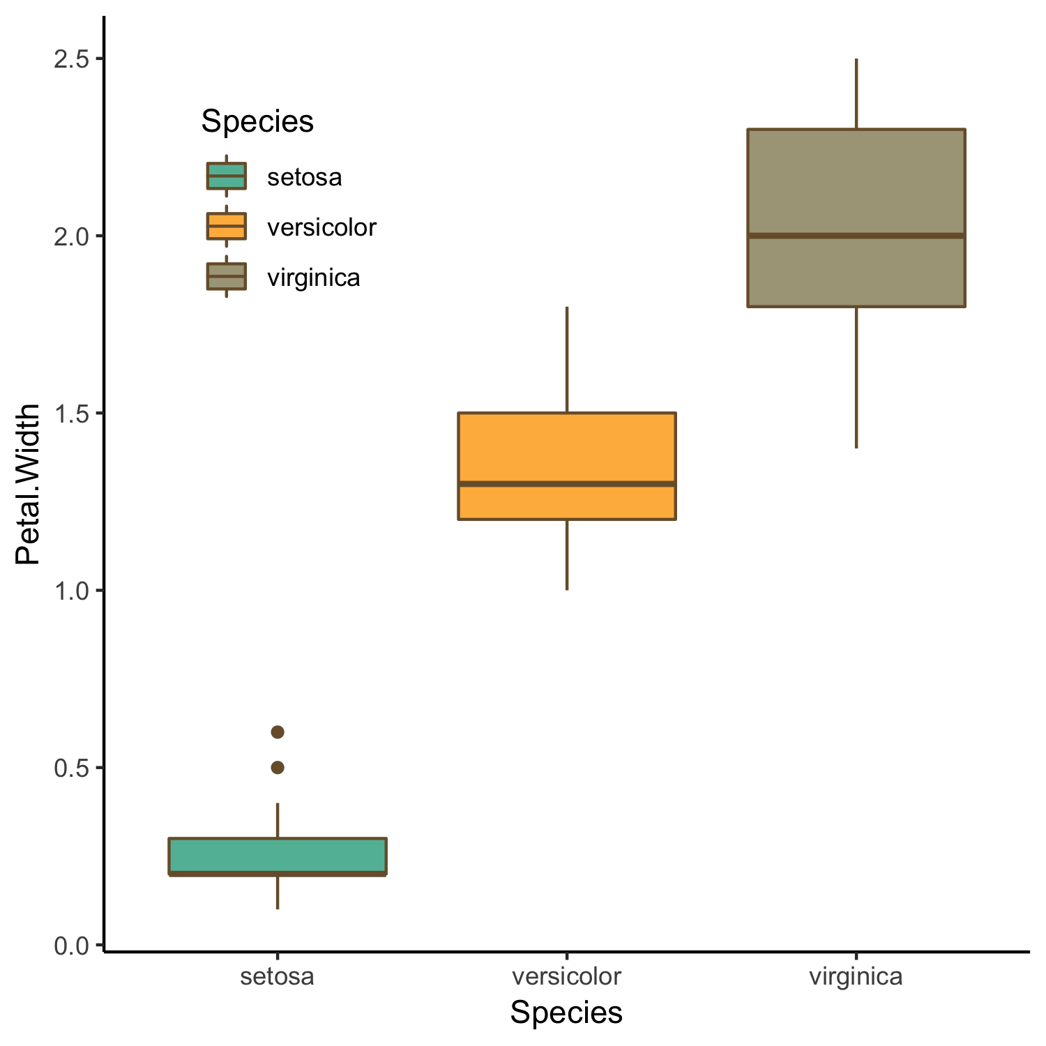
From the above plots we see a visual correlation between plant traits. We can also see that there is some clustering within species with traits varying greatly between the three iris species. Now that we know that there is a clear difference in structural traits between species we could ask the following question:
2. Train your algorithm
Could we predict what species iris plants belong to based on structural trait data alone?
The goal of this tutorial will be to answer this question by building a predictive model and assessing its performance. To do so we will take a random sample of our data which we will use as training data, and another sample which will be used to test our model. These final predictions can then be compared to our original data so we can assess our results and see how accurate our model is.
Building our k-nn classifier
Data normalisation and training/test-set generation
The scales of individual variables may vary with a given dataset. For example one variable may have values ranging from 0 - 1 while the other ranges from 0 - 1000. Therefore some scaling/normalisation is often useful, espescially with the knn algorithm which is quite sensitive to different intervals across variables given that it employs a distance function when searching for ‘nearest-neighbours’.
# Building a normalisation function
normalise <- function(x) {
  num <- x - min(x)
  denom <- max(x) - min(x)
  return (num/denom)
}
For further understanding why feature normalisation is useful see this lecture and/or a very good answer on this topic on StackOverflow. Now we normalise all the continous data columns in the iris dataset by applying our function to the iris data.
iris.norm <- as.data.frame(lapply(iris[1:4], normalise))
Now that our data is normalised, we are going to randomly generate our training and test samples and their respective labels/classes.
This is done using the sample function which generates a random sample of the specified size from the data set or elements. Also note that before calling sample we also call the set.seed function. This ensures that we always generate the same random data sample, as otherwise each time we would run this code a completely new random sequence would be generated. More information on that here.
# Generating seed
set.seed(1234)

# Randomly generating our training and test sampels with a respective ratio of 2/3 and 1/3
datasample <- sample(2, nrow(iris.norm), replace = TRUE, prob = c(0.67, 0.33))

# Generate training set
iris.training <- iris.norm[datasample == 1, 1:4]

# Generate test set
iris.test <- iris.norm[datasample == 2, 1:4]
The next step is to generate our training and test labels. Beware however, we now need to use our original (not-normalised) dataset that also includes our class labels (column 5), while in the previous step we were just interested in our continous variables (columns 1-4). If this is not clear view all datasets again before proceeding.
# Generate training labels
irisTraining.labels <- iris[datasample == 1, 5]

# Generate test labels
irisTest.labels <- iris[datasample == 2, 5]
It’s now time to build our classifier! For this we will use the knn function from the class package. We will pass the function the following parameters:
- Our normalised training dataset
- Our normalised test dataset
- Our original training labels
- A value for K
Note that we also select a value for k, which in this case is 3. By chosing an odd value we avoid a tie between the two classes during the algorithm’s majority voting process.
# Building our knn classifier
iris.knn <- knn(train = iris.training, test = iris.test, cl = irisTraining.labels, k = 3)
3. Assess your model
Next, we need to evaluate the performance of our model. To do this we want to find out if the classes our algorithm predicts based on the training data accurately predict the species classes in our original iris dataset. For this we compare the original class labels to the predictions made by our algorithm.
# creating a dataframe from known (true) test labels
test.labels <- data.frame(irisTest.labels)

# combining predicted and known species classes
class.comparison <- data.frame(iris.knn, test.labels)

# giving appropriate column names
names(class.comparison) <- c("Predicted Species", "Observed Species")
Let’s have a look at how our model did by inspecting the class.comparison table to see if our predicted species align with our observed species.
# inspecting our results table
class.comparison
Finally, we can also evaluate the model using a cross-tabulation or so called contingency table. These are very useful when we wish to understand what correlations exist between different categorical variables. In this case we will be able to tell what classes our model predicted and how those predicted classes compare to the actual iris classes.
CrossTable(x = irisTest.labels, y = iris.knn, prop.chisq = FALSE)
                | iris.knn
irisTest.labels |     setosa | versicolor |  virginica |  Row Total |
----------------|------------|------------|------------|------------|
         setosa |         12 |          0 |          0 |         12 |
                |      1.000 |      0.000 |      0.000 |      0.300 |
                |      1.000 |      0.000 |      0.000 |            |
                |      0.300 |      0.000 |      0.000 |            |
----------------|------------|------------|------------|------------|
     versicolor |          0 |         12 |          0 |         12 |
                |      0.000 |      1.000 |      0.000 |      0.300 |
                |      0.000 |      0.857 |      0.000 |            |
                |      0.000 |      0.300 |      0.000 |            |
----------------|------------|------------|------------|------------|
      virginica |          0 |          2 |         14 |         16 |
                |      0.000 |      0.125 |      0.875 |      0.400 |
                |      0.000 |      0.143 |      1.000 |            |
                |      0.000 |      0.050 |      0.350 |            |
----------------|------------|------------|------------|------------|
   Column Total |         12 |         14 |         14 |         40 |
                |      0.300 |      0.350 |      0.350 |            |
----------------|------------|------------|------------|------------|
To evaluate our algorithm’s performance we can check if there are any discrepancies between our iris.knn model predictions and the actual irisTest.labels. To do this you can first check the total number of predicted classes per category in the last row under column total.
These can then be compared against the actual classes on the right under row total. Our knn model predicted 12 setosa, 14 versicolor and 14 virginica. However when comparing this to our actual data there were 12 setosa, 12 versicolor and 16 virginca species in our test dataset.
Overall we can see that our algorithm was able to almost predict all species classes correctly, except for a case where two samples where falsely classified as versicolor when in fact they belonged to virginica. To improve the model you could now experiment with using different k values to see if this impacts your model results in any way.
Finally now that your model is trained you could go ahead and try to implement your algorithm on the entire iris dataset to see how effective it is!
Summary
In this tutorial we have now covered the following:
- the very basics of machine learning in
R - implementing a k-nearest neighbour classification algorithm
- building our own training and test datasets
- testing and evaluating our knn algorithm using cross-tabulation
However there is still a whole world to explore. For those interested in learning more have a look at this freely available book on machine learning in R.