Tutorial Aims:
All the files you need to complete this tutorial can be downloaded from this repository. Click on Code/Download ZIP and unzip the folder, or clone the repository to your own GitHub account.
In this tutorial, we are going to explore spatial analysis in R using satellite data of the Loch Tay area of Scotland. Satellite or remote-sensing data are increasingly used to answer ecological questions such as what are the characteristics of species’ habitats, can we predict the distribution of species and the spatial variability in species richness, and can we detect natural and man-made changes at scales ranging from a single valley to the entire world.
Around Loch Tay, for instance, remote-sensing data could be used to map different vegetation types, such as invasive species like rhododendron, and track changes over time. Alternatively, satellite data can be used to estimate forest cover for an area like Scotland and help policy makers set new targets and assess progress.
R is a widely used open source programming language for data analysis and visualisation but it is also a powerful tool to explore spatial data. If you are not familiar with R or Rstudio, this introductory tutorial and this troubleshooting tutorial are good starting points.
Working with spatial data can be complicated due to the many different file formats and large size they can have. To simplify this tutorial, we will use a Sentinel 2 satellite image collected on the 27th June 2018 and downloaded from the Copernicus Hub. This website provides free and open access to satellite data, but please note the files are very large and may take some time to download. The image used in this tutorial was cropped to reduced its size and corrected for atmospheric correction in SNAP, the free open source esa toolbox, and saved as a ‘geoTIF’ file (georeferenced image) to make it easier to import. Introductory tutorials for SNAP are availlable here.
Alternatively, for large scale analysis where downloading huge files is not an option, Google Earth Engine is a powerful tool providing an online code editor where users can work with a large selection of databases, whilst harnessing the power of the Google servers. You can find a Google Earth Engine intro tutorial here if you’re interested.
Satellite data mostly consist of reflectance data, which can be defined as a measure of the intensity of the reflected sun radiation by the earth’s surface. Reflectance is measured for different wavelength of the electromagnetic spectrum. The Sentinel 2 optical sensor measures reflectance at 13 wavelength bandwidths, or bands for short. In satellite images, these data are stored in rasters, or a matrix data structure, where each pixel stores the data for the 13 wavelengths. Therefore, Sentinel 2 data contains several raster layers, one for each spectral band. More information on Sentinel 2 can be accessed here.
1. Explore raster data
Once you have unzipped the files you downloaded from the repository on your computer, open RStudio, create a new script by clicking on File/ New File/ R Script. It is always a good idea the write a header to your script with your name, data and purpose such as Intro to spatial analysis tutorial as shown below. Then, set the working directory to the location of the unzipped files on your computer and load the following packages, installing them if necessary:
# Intro to spatial analysis tutorial
# Satellite data available from https://scihub.copernicus.eu/

# Maude Grenier s0804311@ed.ac.uk
# 03-12-2018
##############################################################

# Set the working directory (example, replace with your own file path)
setwd("C:/Users/name/folder/spatialR")

# Load packages

# If you haven't installed the packages before, use e.g.:
# install.packages("sp")

library(sp)
library(rgdal)
library(raster)
library(ggplot2)
library(viridis)
library(rasterVis)
The sp package is central for spatial data analysis in R as it defines a set of classes to represent spatial data. Another important package for spatial analysis is the raster package.
A raster is a grid of equal size cells, or pixels in satellite images, and it is commonly used to represent spatially continuous data. The cells can have one or more values, or even no values for the variable of interest. In the trimmed multispectral image we will be using, each cell contains relfectance data for 12 spectral bands.
The raster package has functions that allow the creation, reading, manipulation and saving of raster data. The package rgdal is used to read or save spatial data files and the package raster uses it behind the scenes.
The package viridis is an aesthetically pleasing colour palette visible to people with colour blindness. We will use it to plot our results as well as ggplot.
First, we will use the raster package to read the satellite image file and inspect its properties.
# Load data
tay <- raster('taycrop.tif')

# Get properties of the Tay raster
tay
In the output, we get details of the image such as the number of bands, dimension (number of rows, columns, and cells), the extent given by the coordinate references, and the coordinate reference system (CRS) which is here the Universal Trans Mercator (UTM) with datum WGS84.
> tay
> class       : RasterLayer
> band        : 1  (of  12  bands)
> dimensions  : 507, 848, 429936  (nrow, ncol, ncell)
> resolution  : 9.217891e-05, 9.217891e-05  (x, y)
> extent      : -4.320218, -4.242051, 56.45366, 56.50039  (xmin, xmax, ymin, ymax)
> coord. ref. : +proj=longlat +datum=WGS84 +no_defs +ellps=WGS84 +towgs84=0,0,0
> data source : C:/Users/maude/Desktop/sentinel2/Taycrop.tif
> names       : Taycrop
We can create individual raster layers for each of the spectral bands in the raster tay.
b1 <- raster('taycrop.tif', band=1)
b2 <- raster('taycrop.tif', band=2)
b3 <- raster('taycrop.tif', band=3)
b4 <- raster('taycrop.tif', band=4)
b5 <- raster('taycrop.tif', band=5)
b6 <- raster('taycrop.tif', band=6)
b7 <- raster('taycrop.tif', band=7)
b8 <- raster('taycrop.tif', band=8)
b9 <- raster('taycrop.tif', band=9)
b10 <- raster('taycrop.tif', band=10)
b11 <- raster('taycrop.tif', band=11)
b12 <- raster('taycrop.tif', band=12)
We can now compare two bands to see if they have the same extent, number of rows and column, projection, resolution and origin. As can be seen below, bands 2 and 3 match.
compareRaster(b2, b3)

# TRUE
Checking the coordinate systems and extents of rasters is a very useful skill - quite often when you have problems with working with multiple raster objects, it’s because of differences in coordinate systems or extents.
The bands can be plotted using the plot or image function. Note that the plot function only plots 100,000 pixels
but image strectches the view.
plot(b8)

image(b8)
plot(b8)
zoom(b8)    # run this line, then click twice on your plot to define a box
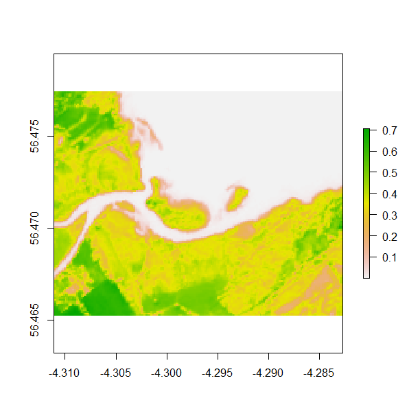
Alternatively, an extent can be cropped and plotted from the plot image using the same double click method described above and the code below. Zooming in allows you to visualise spatial data for specific areas you might be interested in.
plot(tay)
e <- drawExtent()    # run this line, then click twice on your plot to define a box
cropped_tay <- crop(b7, e)
plot(cropped_tay)
2. Visualise spectral bands
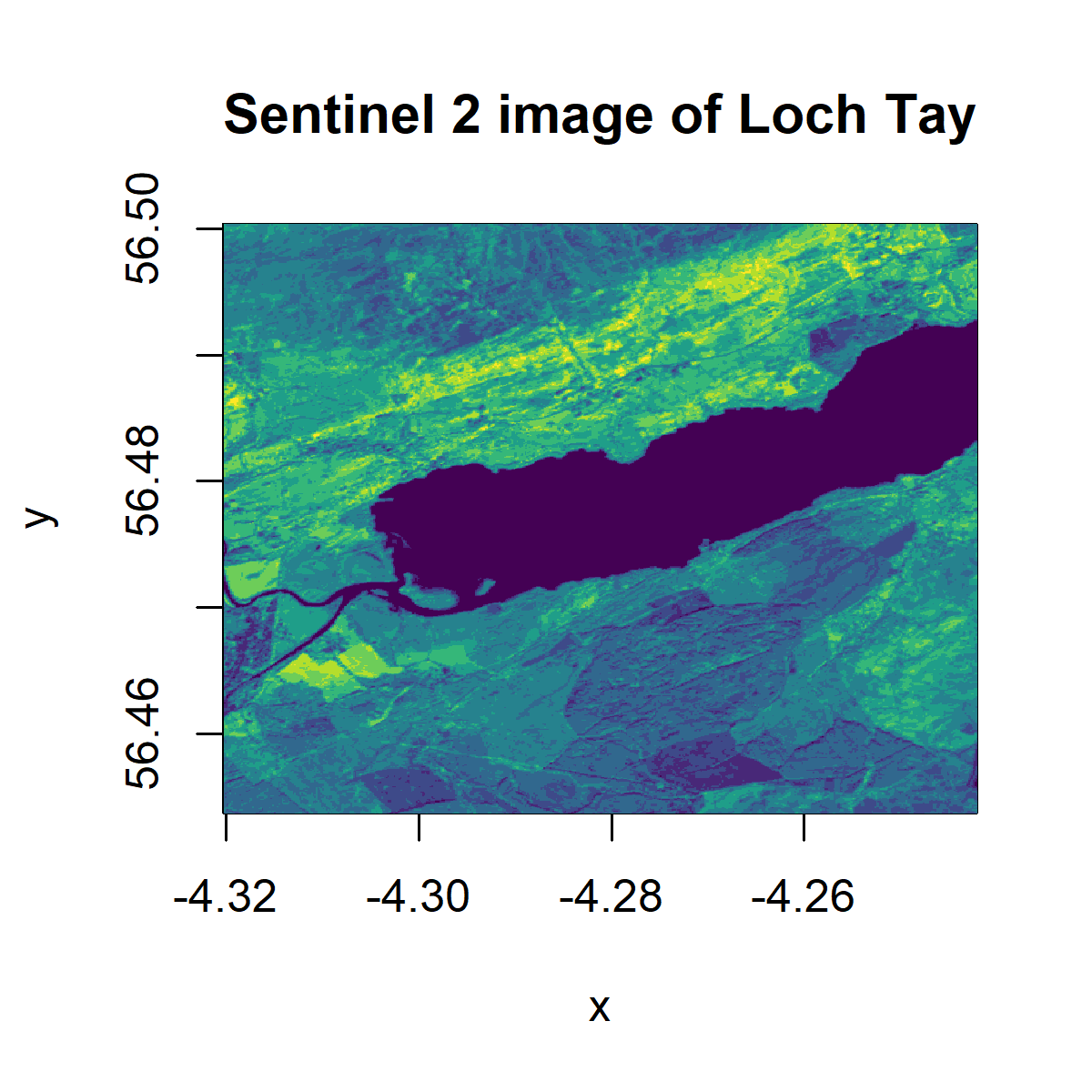
The bands can be plotted with different colour palettes to improve visualisation, such as viridis, and saved using the code below.
png('tayplot.png', width = 4, height = 4, units = "in", res = 300)                	# to save plot
image(b8, col= viridis_pal(option="D")(10), main="Sentinel 2 image of Loch Tay")
dev.off()         									# to save plot
# dev.off() is a function that "clears the slate" - it just means you are done using that specific plot
# if you don't dev.off(), that can create problems when you want to save another plot
To view the plot without saving the image, you only need the second line:
image(b8, col= viridis_pal(option="D")(10), main="Sentinel 2 image of Loch Tay")
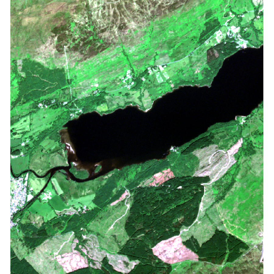
A useful way to visualise the satellite data is to plot a red-green-blue plot of a multi-layered object for a more realistic rendition. The layers or bands represent different bandwidth in the visible electromagnetic spectrum (corresponding to red, blue and green) and combined, create a naturalistic colour rendition of the earth surface.
First, we will create a raster stack, a multi-layered raster object, of the red(b4), green(b3) and blue(b2) bands.
# this code specifies how we want to save the plot
png('RGB.png', width = 5, height = 4, units = "in", res = 300)
tayRGB <- stack(list(b4, b3, b2))              # creates raster stack
plotRGB(tayRGB, axes = TRUE, stretch = "lin", main = "Sentinel RGB colour composite")
dev.off()
Another popular way to visualise remote sensing data is using a false colour composite (FCC), where the red, green, and blue bands have been replaced in order to accentuate vegetation.
In a FCC, the red bands is replaced by the near infrared band (band 8 in Sentinel 2), the green band by red and the blue band by green. This creates an image where the vegetation stands out in red. Check (help(plotRGB)) for more information and other arguments for the function.
Exercise: Create a FCC of the Loch Tay area using a raster stack.
The package rasterVis provides a number of ways to enhance the visualisation and analysis of raster data, as can be seen on the package’s website here. The function levelplot allows level and contour plots to be made of raster objects with elevation data, such as LIDAR and plot3D allows 3D mapping. We do not have elevation data from Sentinel 2, but the package’s gplot function allows us to plot a uni or multivariate raster object using ggplot2 like syntax.
For an introduction to the ggplot2 package, check out our tutorial here or you can find a cheatsheet here.
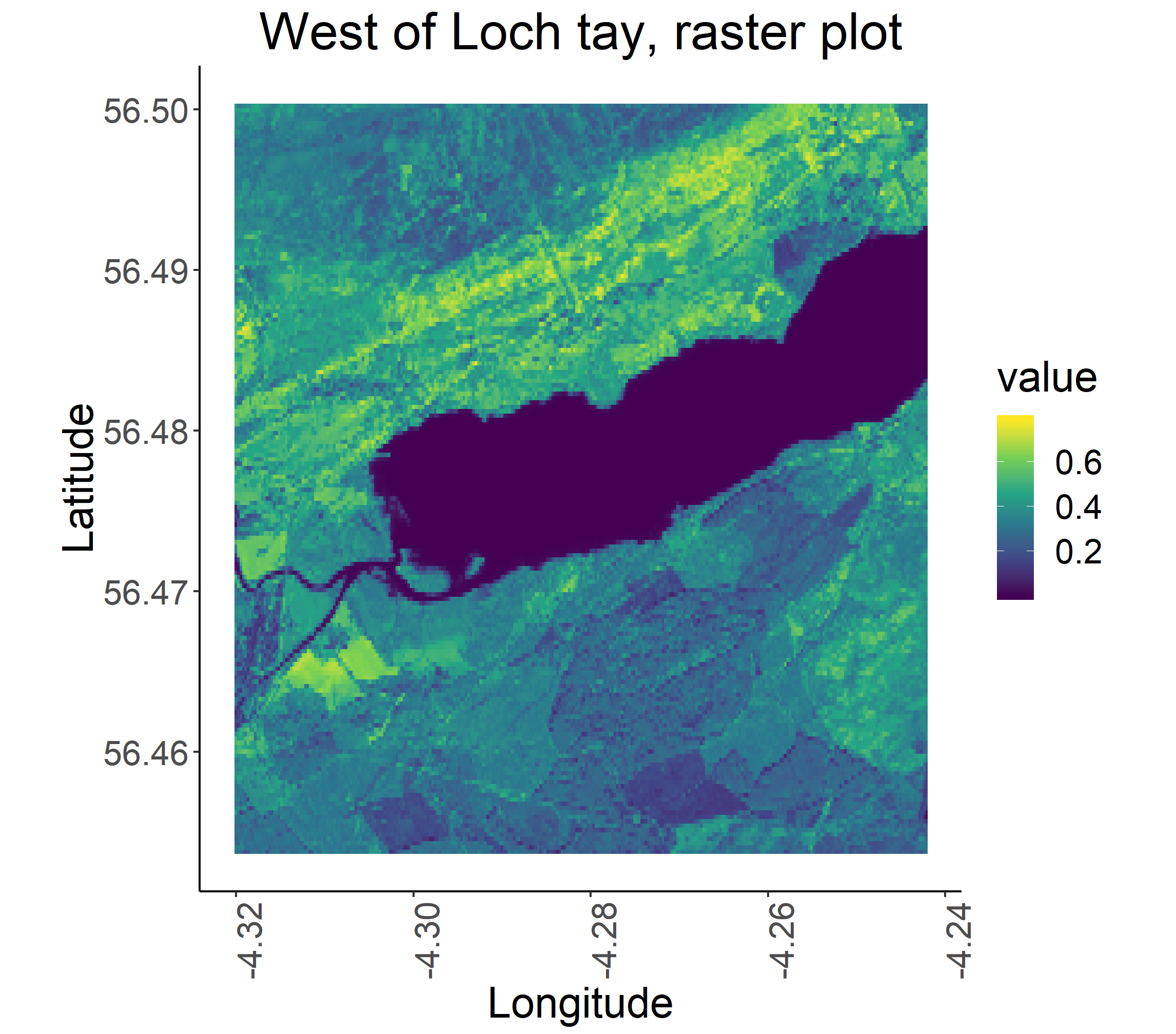
gplot(b8) +
  geom_raster(aes(x = x, y = y, fill = value)) +
  # value is the specific value (of reflectance) each pixel is associated with
  scale_fill_viridis_c() +
  coord_quickmap() +
  ggtitle("West of Loch tay, raster plot") +
  xlab("Longitude") +
  ylab("Latitude") +
  theme_classic() +   					    # removes defalut grey background
  theme(plot.title = element_text(hjust = 0.5),             # centres plot title
        text = element_text(size=20),		       	    # font size
        axis.text.x = element_text(angle = 90, hjust = 1))  # rotates x axis text

ggsave("ggtay.png", scale = 1.5, dpi = 300) 		# to save plot
Note that here we saved the plot in a slightly different way - for plots creates using ggplot2, we can use the ggsave function and we define the specifics of the saved plot after we’ve created it, whereas earlier in the tutorial when we were using the png() function in combination with dev.off(), the plot characteristics are defined before we make the plot inside the png() function.
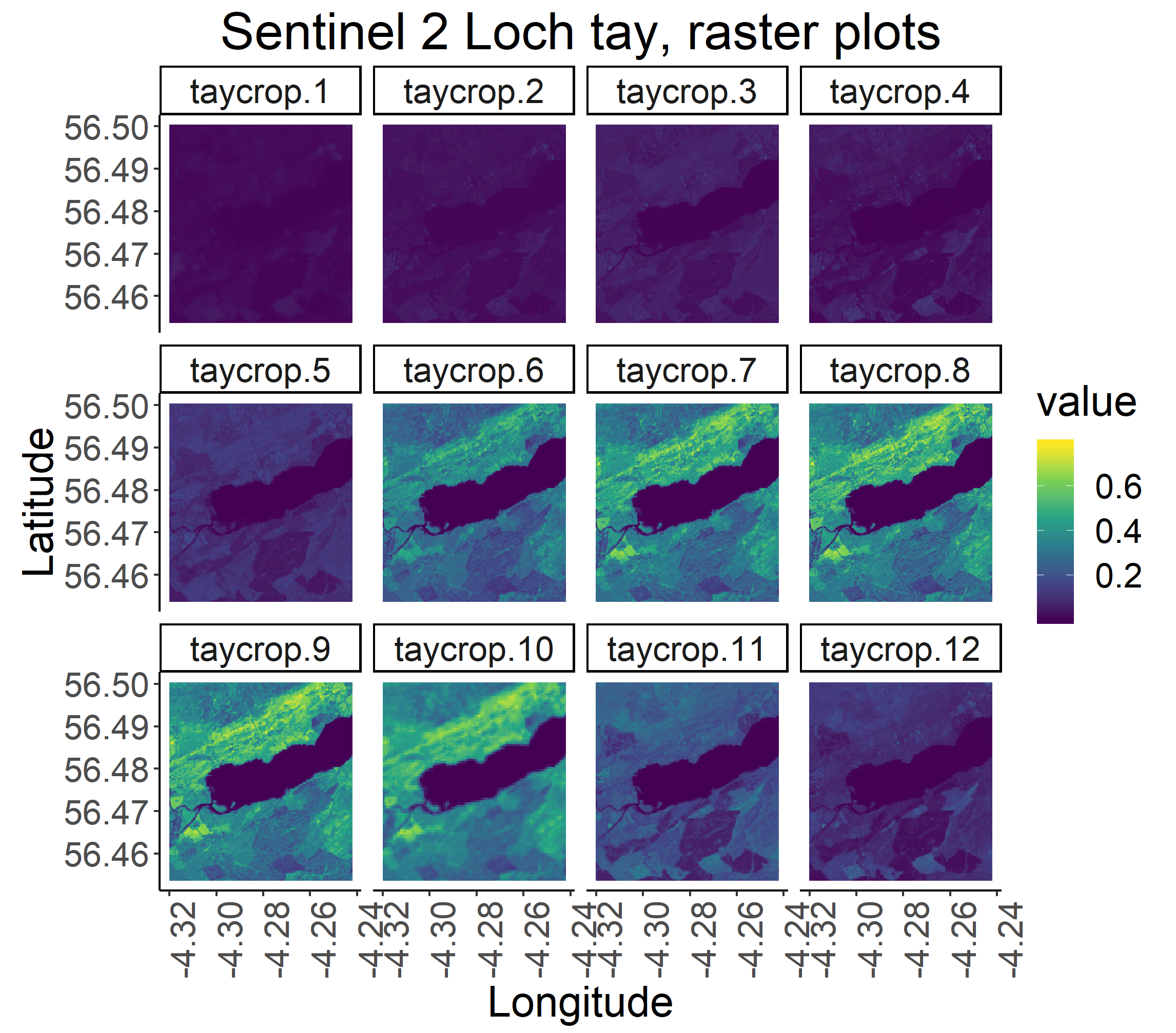
To visualise all the bands together, we can use facet_wrap in gplot. First, we will create a stack of all the bands, so just putting them all on top of each other, like layers in a cake.
t <- stack(b1,b2, b3, b4, b5, b6, b7, b8, b9, b10, b11, b12)
Now we are ready to make out facetted plots.
gplot(t) +
  geom_raster(aes(x = x, y = y, fill = value))+
  scale_fill_viridis_c() +
  facet_wrap(~variable) +
  coord_quickmap()+
  ggtitle("Sentinel 2 Loch tay, raster plots") +
  xlab("Longitude") +
  ylab("Latitude") +
  theme_classic() +
  theme(text = element_text(size=20),
        axis.text.x = element_text(angle = 90, hjust = 1)) +
  theme(plot.title = element_text(hjust = 0.5))

ggsave("allbands.png", scale = 1.5, dpi = 300) # to save plot
Alternatively, for a quick visualisation, the original file can be loaded as a raster brick and plotted using ‘plot’.
s_tay <- brick('taycrop.tif')
plot(s_tay)
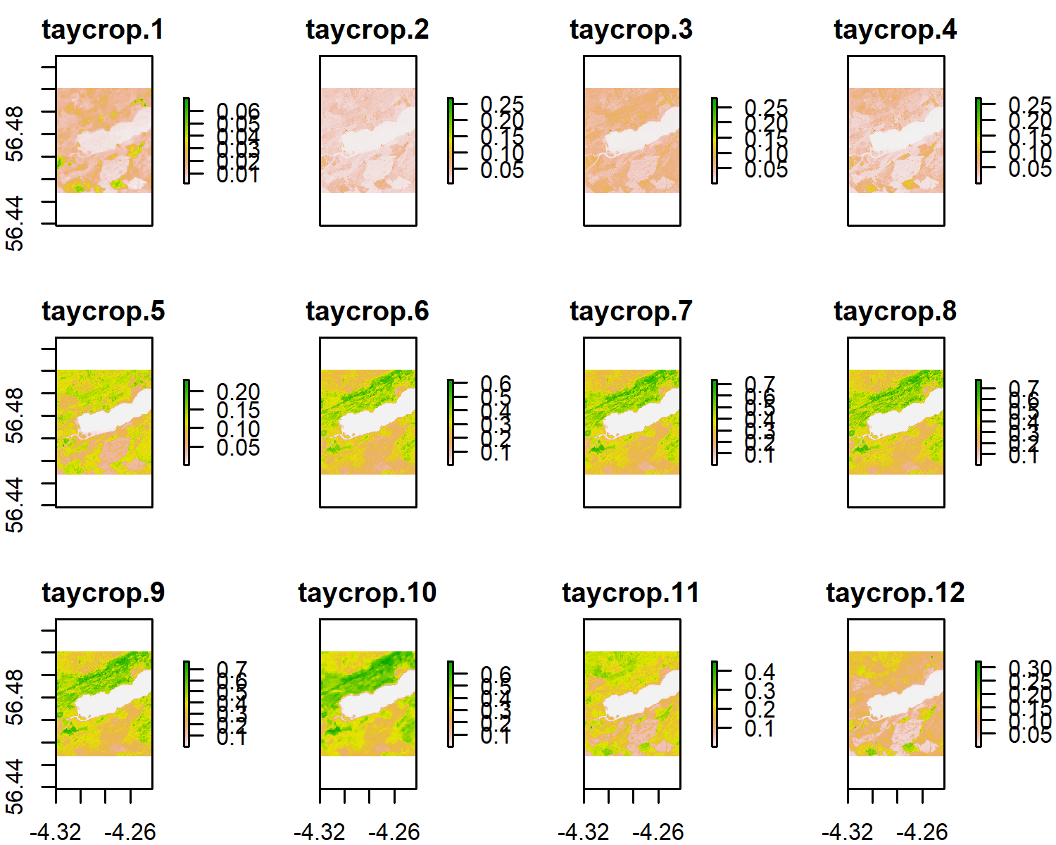
Notice the difference in colour and range of legend between the different bands. Different earth surfaces reflect the solar radiation differently and each raster layer represents how much incident solar radiation is reflected at a particular wavelength bandwidth. Bands 6 to 9 are in the Near Infrared Range (NIR). Vegetation reflects more NIR than other wavelengths but water absorbs NIR, therefore the lighter areas with high reflectance values are likely to be vegetation and the dark blue, low reflectance value areas, likely to be water. Also note that the Sentinel 2 bands have 3 levels of spatial resolution, 10 m, 20 m, and 60 m (see summary below).
10 m resolution band 2, band 3, band 4 and band 8
20 m resolution band 5, band 6, band 7, band 11 and band 12
60 m resolution band 1, band 9 and band 10
3. Manipulate rasters: NDVI and KMN classification
The Normalised Difference Vegetation Index (NDVI) is a widely used vegetation index that quantifies vegetation presence, health or structure. It is calculated using the Near Infrared (NIR) and Red bandwith of the spectrum. Healthy vegetation reflects light strongly in the NIR part of the spectrum and absorbs light in red part of the visible spectrum for photosynthesis. A high ratio between light refected in the NIR part of the spectrum and light reflected in the red part of the spectrum would represent areas that potentially have healthy vegetation. It is worth noting that different plant species absorb light in the red part of the spectrum at different rates. The same plant will also absorb light in the red band differently depending on whether it is stressed or healthy, or the time of year. It is often used over large areas as an indication of land cover change.
The NDVI ratio is calculated using (NIR - Red) / (NIR + Red). For example, a pixel with an NDVI of less than 0.2 is not likely to be dominated by vegetation, and an NDVI of 0.6 and above is likely to be dense vegetation.
In R, we can calculate the NDVI by creating a function and using raster math operations where NIR = band 8 and Red = band 4 in Sentinel 2 images. We will first use the raster brick we created earlier from the original file.
# NDVI

# Created a VI function (vegetation index)
VI <- function(img, k, i) {
  bk <- img[[k]]
  bi <- img[[i]]
  vi <- (bk - bi) / (bk + bi)
  return(vi)
}

# For Sentinel 2, the relevant bands to use are:
# NIR = 8, red = 4
Now we are ready to apply our function to the raster we’ve been working with so far!
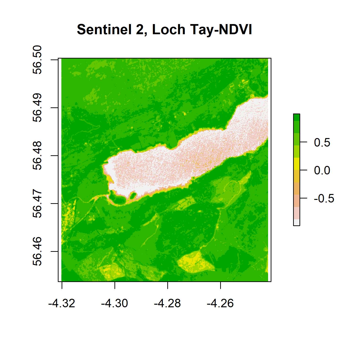
ndvi <- VI(s_tay, 8, 4)
# 8 and 4 refer to the bands we'll use

png('ndviplot.png', width = 4, height = 4, units = "in", res = 300)
plot(ndvi, col = rev(terrain.colors(10)), main = 'Sentinel 2, Loch Tay-NDVI')
dev.off()
To find out the distribution of the pixel NDVI values, we can plot a histogram.
# Create histogram of NDVI data

png('ndvihist.png', width = 4, height = 4, units = "in", res = 300)
hist(ndvi,
     main = "Distribution of NDVI values",
     xlab = "NDVI",
     ylab= "Frequency",
     col = "aquamarine3",
     xlim = c(-0.5, 1),
     breaks = 30,
     xaxt = 'n')
axis(side = 1, at = seq(-0.5,1, 0.05), labels = seq(-0.5,1, 0.05))
dev.off()
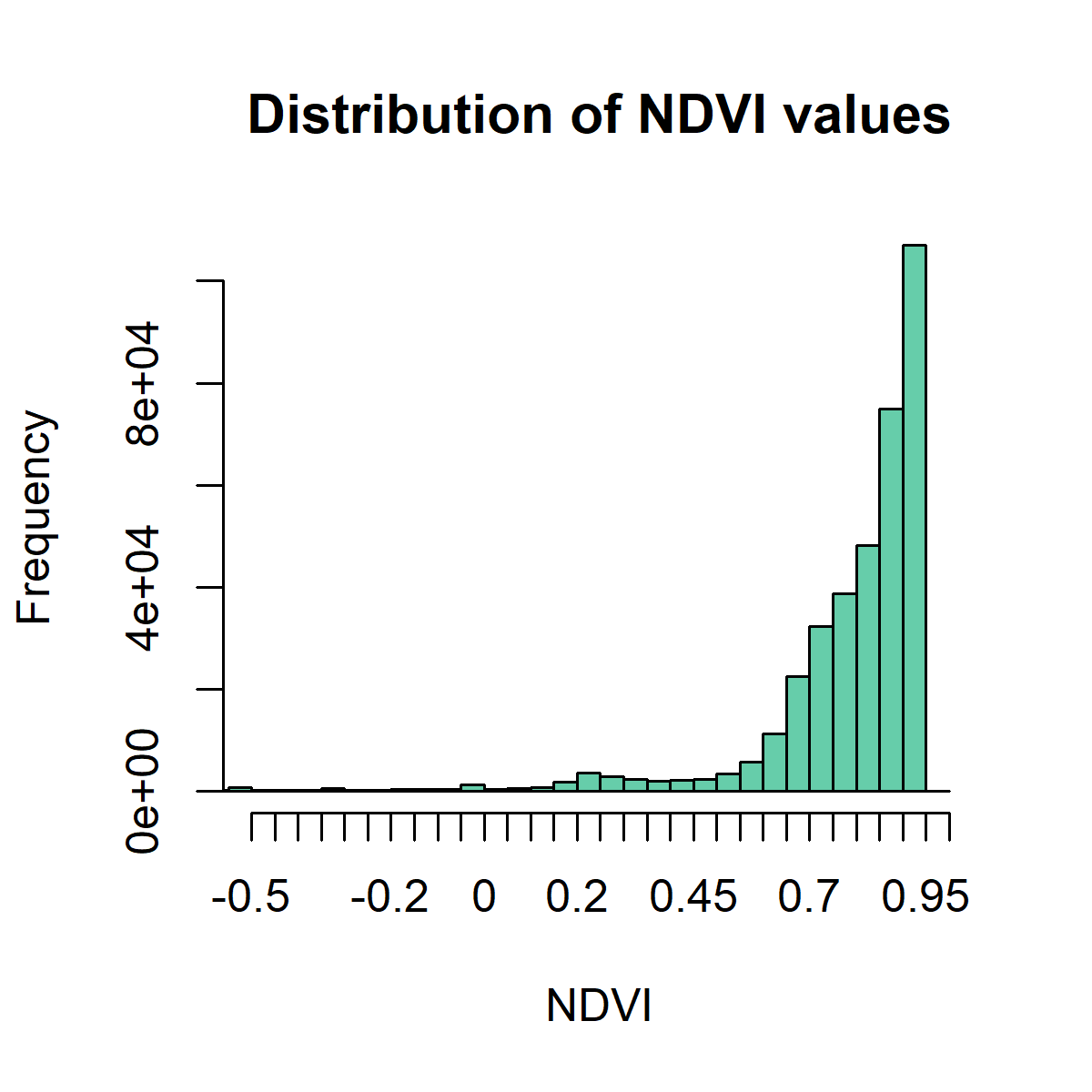
So what does this mean?
The histogram is strongly skewed to the right, towards highh NDVI values, indicating a highly vegetated area.
Now that we know that this area has lots of vegetation, we can also mask the pixels with an NDVI value of less than 0.4 (less likely to be vegetation) to highlight where the vegetated areas occur.
# Mask cells that have NDVI of less than 0.4 (less likely to be vegetation)

png('ndvimask.png', width = 4, height = 4, units = "in", res = 300)

veg <- reclassify(ndvi, cbind(-Inf, 0.4, NA))
# We are reclassifying our object and making all values between
# negative infinity and 0.4 be NAs

plot(veg, main = 'Veg cover')
dev.off()
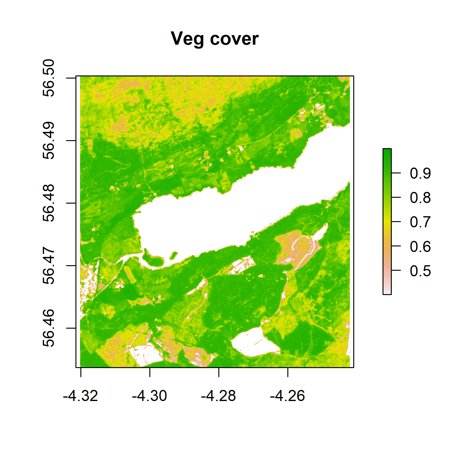
We still have a high vegetation cover, which is to be expected in this part of Scotland.
How can we save the raster itself, not just plots?
We might want to export the NDVI raster we just created to use in QGIS or other software, or to save it for further use in R.
To save a raster object, use the writeraster function. Saving the data as integers rather than floats requires less memory and processing for the computer to handle. A float is a term used to describe a variable with a fractional value or decimals, e.g. 0.002.
writeRaster(x = ndvi,

            # where your file will go - update with your file path!

            filename="yourepo/sentinel2/tay_ndvi_2018.tif",
            format = "GTiff", 					# save as a tif
            datatype = 'INT2S') 					# save as a INTEGER rather than a float
Raster operations also allow us to perform an unsupervised classification, or a clustering of the pixels, in the satellite image. In this context, unsupervised means that we are not using training data for the clustering.
This type of classification can be useful when not a lot is known about an area. In the example below, we are going to use the kmeans algorithm. The algorithm groups pixels that have similar spectral properties in the same cluster. We are going to create 10 clusters using the NDVI raster we have just created above, but first, we need to convert the raster into an array, which is the object format required for the classification.
# convert the raster to vector/matrix ('getValues' converts the RasterLAyer to array) )

nr <-getValues(ndvi)
str(nr)

# important to set the seed generator because `kmeans` initiates the centres in random locations
# the seed generator just generates random numbers

set.seed(99)

# create 10 clusters, allow 500 iterations, start with 5 random sets using 'Lloyd' method

kmncluster <- kmeans(na.omit(nr), centers = 10, iter.max = 500,
                     nstart = 5, algorithm = "Lloyd")

# kmeans returns an object of class 'kmeans'

str(kmncluster)
Kmeans returns an object with 9 elements. The length of the cluster element within kmncluster is 429936
which is the same as the length of nr created from the ndvi object. The cell values of kmncluster$cluster range between 1 to 10 corresponding to the input number of clusters we provided in the kmeans() function. kmncluster$cluster indicates
the cluster label for the corresponding pixel.
Our classification is now complete, and to visualise the results, we need to convert the kmncluster$cluster array back to a RasterLayer of the same dimension as the ndvi object.
# First create a copy of the ndvi layer
knr <- ndvi

# Now replace raster cell values with kmncluster$cluster
# array
knr[] <- kmncluster$cluster

# Alternative way to achieve the same result
values(knr) <- kmncluster$cluster
knr
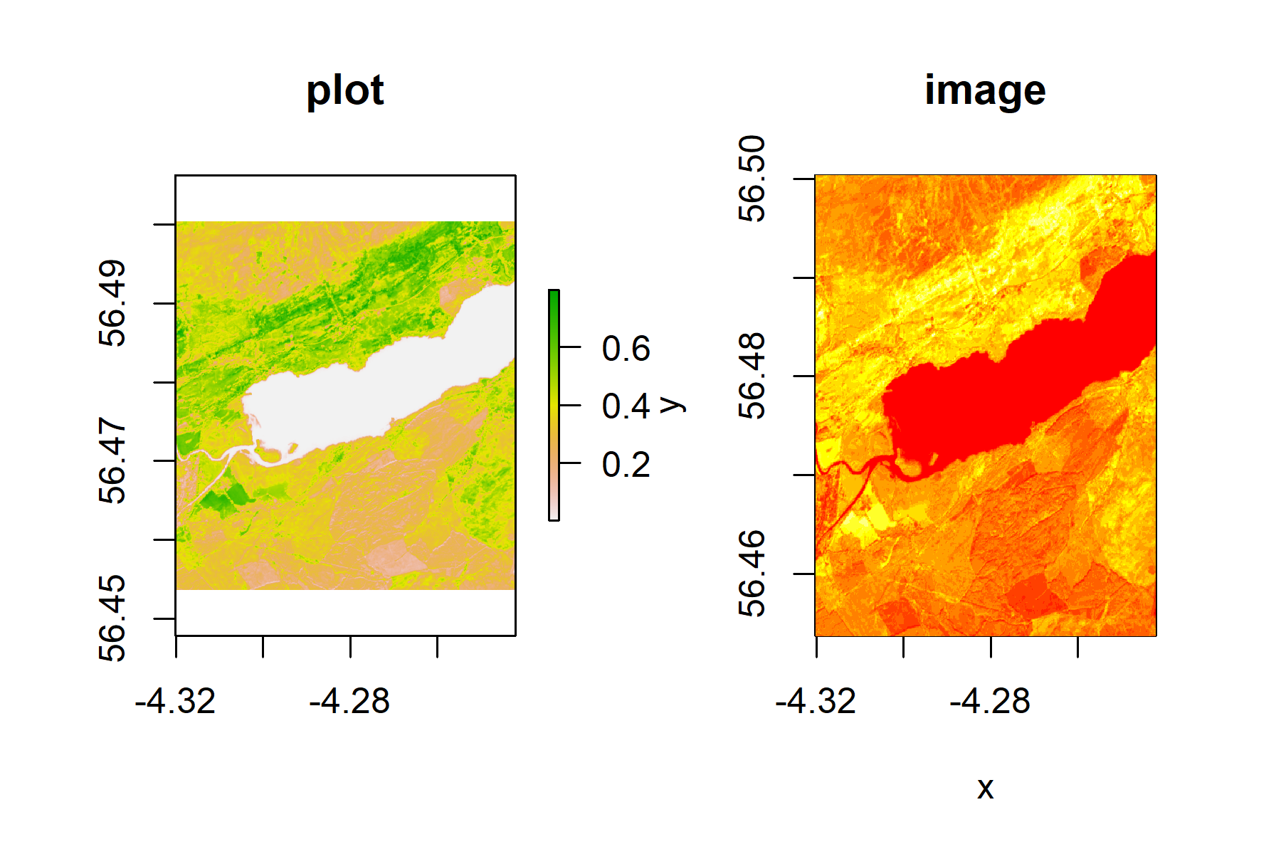
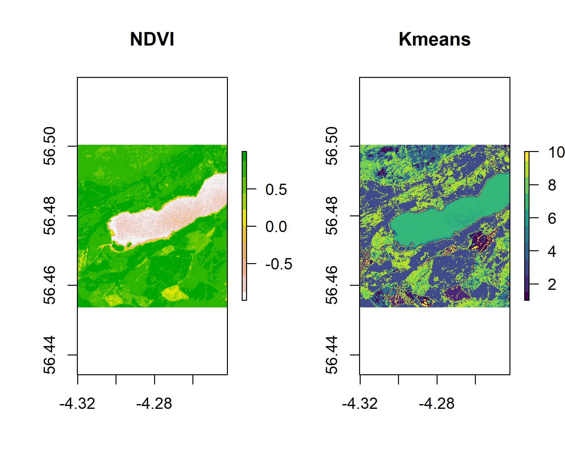
We can see that knr is a RasterLayer with 429,936 cells, but we do not know which cluster (1-10) belongs what land cover or vegetation type. One way of attributing a class to a land cover type is by plotting the cluster side-by-side with a reference layer of land cover and using unique colours for each cluster. As we don’t have one for our example area, we can use the NDVI map we created earlier or the RGB plot.
par(mfrow = c(1, 2))
plot(ndvi, col = rev(terrain.colors(10)), main = "NDVI")
plot(knr, main = "Kmeans", col = viridis_pal(option = "D")(10))
If we want to plot our classification alongside the RGB rendering of the raster, and save the two plots, we can use the code below:
png('rgb_kmeans.png', width = 10, height = 8, units = "in", res = 300)
par(mar = c(10.8, 5, 10.8, 2), mfrow = c(1, 2))
plotRGB(tayRGB, axes = TRUE, stretch = "lin", main = "RGB")
plot(knr, main = "Kmeans", yaxt = 'n', col = viridis_pal(option = "D")(10))
dev.off()
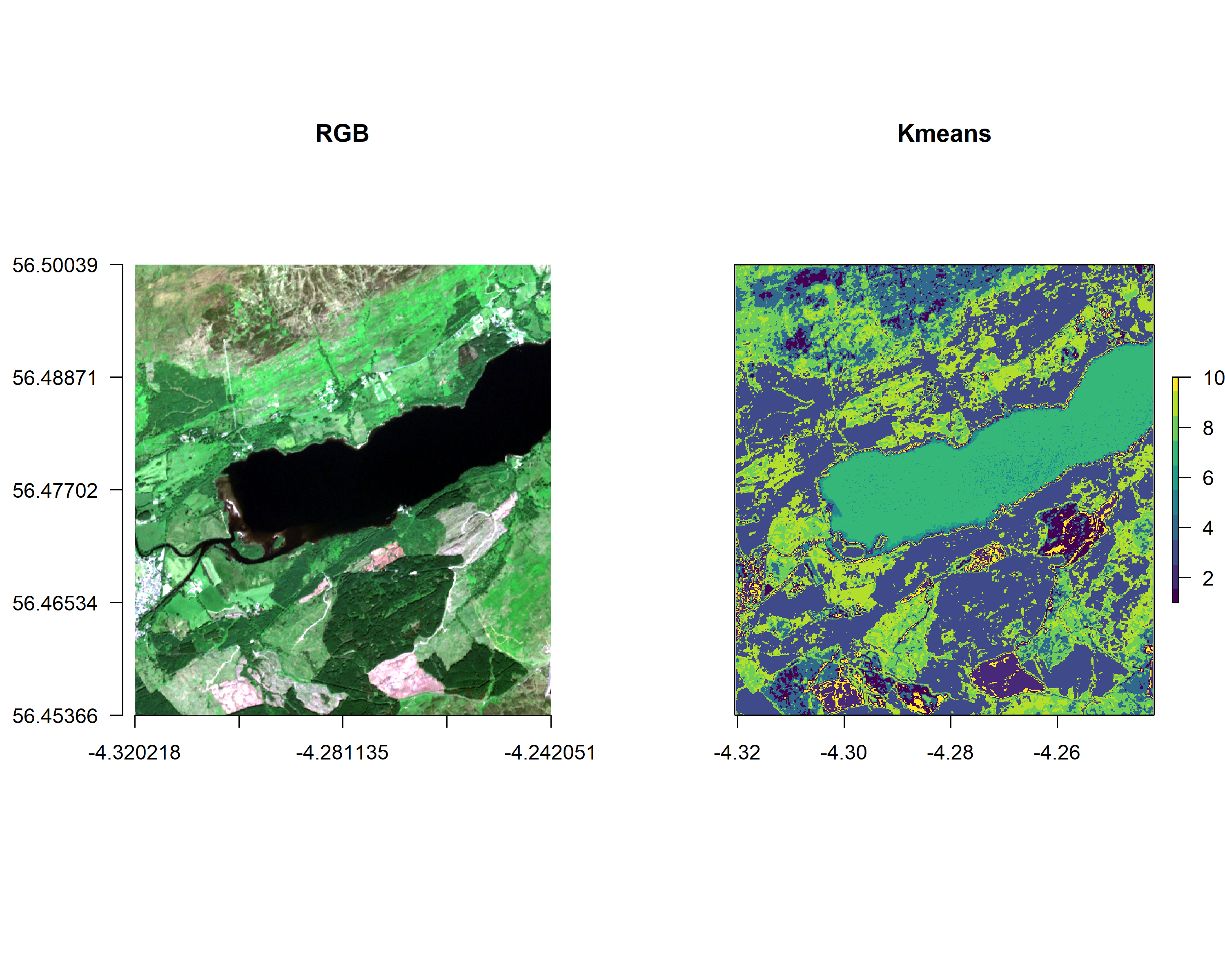
A simple classification like this one is only to give an idea of land cover types. In the above example, we could deduce that cluster 8, in green, is water as it covers the Loch. We can also spot patterns in the vegetation cover in both the NDVI and kmeans cluster plots. We could deduce that the areas with the highest NDVI ratio are likely to be forest cover.
Exercise: Using the NDVI, RGB and kmeans plot, can you deduce other land cover around the Loch Tay area?
Conclusion
In this introduction to remote sensing spatial analysis, we have covered how to:
- Import a GeoTIFF file as a raster in R.
- Extract layers from a multi-layer raster objects and get the raster properties.
- Explore raster visulaisation of single and mutil-layered object with rasterVis, ggplot and base R.
- Explore raster manipulations by calculating and plotting the NDVI ratio of the pixels in our image.
- Perform an unsupervised image classification using the kmeans algorithm to cluster the pixels in 10 clusters.
If you want to explore further, there are excellent resources availabe in the Spatial Data Science with R by Robert J. Hijmans.
Doing this tutorial as part of our Data Science for Ecologists and Environmental Scientists online course?
This tutorial is part of the Stats from Scratch stream from our online course. Go to the stream page to find out about the other tutorials part of this stream!
If you have already signed up for our course and you are ready to take the quiz, go to our quiz centre. Note that you need to sign up first before you can take the quiz. If you haven't heard about the course before and want to learn more about it, check out the course page.