Created by John

Tutorial aims:

1. Downloading Shiny
2. Getting familiar with the Shiny app file structure
3. Getting familiar with the Shiny app.R layout
4. Creating a Shiny app
5. Exporting a finished app
6. Challenge yourself to write an app

At it’s core, Shiny is merely an R package like dplyr or ggplot2. The package is used to create web-applications, but uses the R language rather than javascript or HTML5, which are traditionally used for web applications. By using R, Shiny provides an efficient method of creating web applications designed around data presentation and analysis.

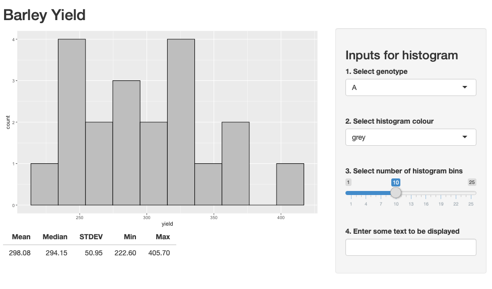
Below is an example of the basic Shiny app that we will be recreating in today’s tutorial:

Have a look at these examples if you want to see what a Shiny app looks like, or if you want inspiration for your own app.

What are Shiny Apps useful for?

• Interactive data visualisation for presentations and websites
• Sharing results with collaborators
• Communicating science in an accessible way
• Bridging the gap between R users and non-R users

1. Downloading Shiny and tutorial resources

To get Shiny in RStudio, the first thing you need is the shiny package, by running the code below in RStudio:

install.packages("shiny")
install.packages("rsconnect")  # For publishing apps online
install.packages("agridat")  # For the dataset in today's tutorial

2. The Shiny app file structure

Next, select File/ New File/ Shiny Web App…, give the application a descriptive name (no spaces) and change the application type to “Single File (app.R)”, save the app in an appropriate directory and click Create.

RStudio generates a template R script called app.R. Delete all the code in the template so you have a blank script.

Notice that the name you gave to your app was assigned to the directory, not the app script file. For your app to work, the file must remain named app.R!

It is possible to create a Shiny app with two files called ui.R and server.R, but the same can be accomplished by using one file. In the past, Shiny apps had to be created using two files, but the Shiny package has since been updated to allow the single file app structure, making things much tidier. You will see some tutorials on the internet using the old two file structure, but these can be easily translated to the one file structure. This tutorial will assume you have the one file app structure.

Now we can set up the rest of the folders for your app. Add a folder called Data and a folder called www in your app directory. Data will hold any data used by the app and www will hold any images and other web elements.

To review, a Shiny application should have this specific folder structure to work properly:

Test_App
├── app.R
├── Data
│   └── data.csv
└── www
    └── A.jpg

3. app.R layout

Now that the folder structure is set up, head back to RStudio to start building app.R. A basic app.R consists of these five parts:

• A section at the top of the script loading any packages needed for the app to run. shiny is required at the very least, but others like dplyr or ggplot2 could be added as they are needed:

# Packages ----
library(shiny)  # Required to run any Shiny app
library(ggplot2)  # For creating pretty plots
library(dplyr)  # For filtering and manipulating data
library(agridat)  # The package where the data comes from

• A section loading any data needed by the app:

# Loading data ----
Barley <- as.data.frame(beaven.barley)

• An object called ui, which contains information about the layout of the app as it appears in your web browser. fluidPage() defines a layout that will resize according to the size of the browser window. All the app code will be placed within the brackets.

# ui.R ----
ui <- fluidPage()

• An object called server, which contains information about the computation of the app, creating plots, tables, maps etc. using information provided by the user. All the app code will be placed within the curly brackets.

# server.R ----
server <- function(input, output) {}

• A command to run the app. This should be included at the very end of app.R. It tells shiny that the user interface comes from the object called ui and that the server information (data, plots, tables, etc.) comes from the object called server.

# Run the app ----
shinyApp(ui = ui, server = server)

Delete any example code generated automatically when you created app.R and create a basic Shiny app by copying the snippets of code above into your app.R. Your script should now look like this:

 # Packages ----
 library(shiny)  # Required to run any Shiny app
 library(ggplot2)  # For creating pretty plots
 library(dplyr)  # For filtering and manipulating data
 library(agridat)  # The package where the data comes from

 # Loading data ----
 Barley <- as.data.frame(beaven.barley)

 # ui.R ----
 ui <- fluidPage()

 # server.R ----
 server <- function(input, output) {}

 # Run the app ----
 shinyApp(ui = ui, server = server)

Layout of a Shiny App

Shiny apps are structured using panels, which are laid out in different arrangements. Panels can contain text, widgets, plots, tables, maps, images, etc.

Here is a good set of examples on how the panel layout can be changed. The most basic layout uses fluidRow() and column() to manually create grids of a given size. fluidRow() allows a lot of customisation, but is more fiddly. In this tutorial, we will be using sidebarLayout(), which creates a large panel and a smaller inset side panel.

4. Creating a Shiny App - Basic Syntax

To illustrate how to code a Shiny app, we will recreate a simple app that I wrote to explore some data on the productivity of Barley genotypes.

You can get the code for this app by opening app.R in the Example_app folder in the tutorial repository which you downloaded earlier.

Looking at the app and comparing to the panel layout examples in the above link, we can see that the app has a sidebarLayout with a sidebarPanel, mainPanel and titlePanel. It uses a selectInput to choose the genotype of barley shown in the histogram and the table, another selectInput for the colour of the histogram, a sliderInput to choose the number of bins in the histogram and a textInput to display some text in the app. The histogram is located in the mainPanel along with a summary table of the data being shown, while the inputs are in the sidebarPanel.

Go back to your app.R and fill in the code you already have with the new bits of code below, which will serve as the basic skeleton for our app. Remember that you should only have one ui and one server object. Don’t just copy and paste the below:

# Packages ----
library(shiny)  # Required to run any Shiny app
library(ggplot2)  # For creating pretty plots
library(dplyr)  # For filtering and manipulating data
library(agridat)  # The package where the data comes from

# Loading data ----
Barley <- as.data.frame(beaven.barley)

# ui.R ----
ui <- fluidPage(
  titlePanel(""),  # Add a title panel
  sidebarLayout(  # Make the layout a sidebarLayout
    sidebarPanel(),  # Inside the sidebarLayout, add a sidebarPanel
    mainPanel()  # Inside the sidebarLayout, add a mainPanel
  )
)

# server.R ----
server <- function(input, output) {}

# Run the app ----
shinyApp(ui = ui, server = server)

titlePanel() indicates that we would like a separate panel at the top of the page in which we can put the title.

sidebarLayout() indicates that we want our Shiny app to have the sidebar layout, one of many layouts we saw above. Within sidebarLayout we have:

sidebarPanel() indicates that we want a sidebar panel included in our app. Sidebar panels often contain input widgets like sliders, text input boxes, radio buttons etc.

mainPanel() indicates that we want a larger main panel. Main panels often contain the output of the app, whether it is a table, map, plot or something else.

Input widgets

Now that we have our basic structure we can start to fill it with inputs and outputs.

The example app has four input widgets, a selectInput for genotype, a selectInput for histogram colour, a sliderInput for number of bins and a textInput to add some arbitrary text. Each of these widgets provides information on how to display the histogram and its accompanying table. In the example app, all the widgets are found in the sidebarPanel so the code for these widgets should be put in the sidebarPanel command like this:

ui <- fluidPage(
  titlePanel("Barley Yield"),
  sidebarLayout(
    sidebarPanel(
      selectInput(inputId = "gen",  # Give the input a name "genotype"
      label = "1. Select genotype",  # Give the input a label to be displayed in the app
      choices = c("A" = "a","B" = "b","C" = "c","D" = "d","E" = "e","F" = "f","G" = "g","H" = "h"), selected = "a"),  # Create the choices that can be selected. e.g. Display "A" and link to value "a"
    selectInput(inputId = "colour", 
      label = "2. Select histogram colour", 
      choices = c("blue","green","red","purple","grey"), selected = "grey"),
    sliderInput(inputId = "bin", 
      label = "3. Select number of histogram bins", 
      min=1, max=25, value= c(10)),
    textInput(inputId = "text", 
      label = "4. Enter some text to be displayed", "")
    ),
  mainPanel()
  )
)

Note that choices = c("A" = "a" ... could be replaced with choices = unique(Barley$gen) to simply use the groups directly from the dataset.

Spend a couple of minutes looking at this code so you understand what it means, then fill in your own app.R with the code.

Let’s break down selectInput() to understand what is going on:

• inputId = "genotype" gives this input the name genotype, which will become useful when referencing this input later in the app script.
• label = "1\. Select genotype" gives this input a label to be displayed above it in the app.
• choices = c("A" = "a","B" = "b", ... gives a list of choices to be displayed in the dropdown menu (A, B, etc.) and the value that is actually gathered from that choice for use in the output (a, b, etc.).
• selected = "grey" gives the value from the dropdown menu that is selected by default.

You can look into the arguments presented by the other input widgets by using the help function ?. For example, by running the code ?textInput in the R console.

More Input Widgets

There are plenty of pre-made widgets in Shiny. Here is a selection, each with the minimum number of arguments needed when running the app, though many more can be added:

actionButton(inputId = "action", label = "Go!")

radioButtons(inputId = "radio", label = "Radio Buttons", choices = c("A", "B"))

selectInput(inputId = "select", label = "select", choices = c("A", "B"))

sliderInput(inputId = "slider", label = "slider", value = 5, min = 1, max = 100)

Notice how all of the inputs require an inputId and a label argument.

Running a Shiny App

Take this opportunity to preview your app by clicking Run App:

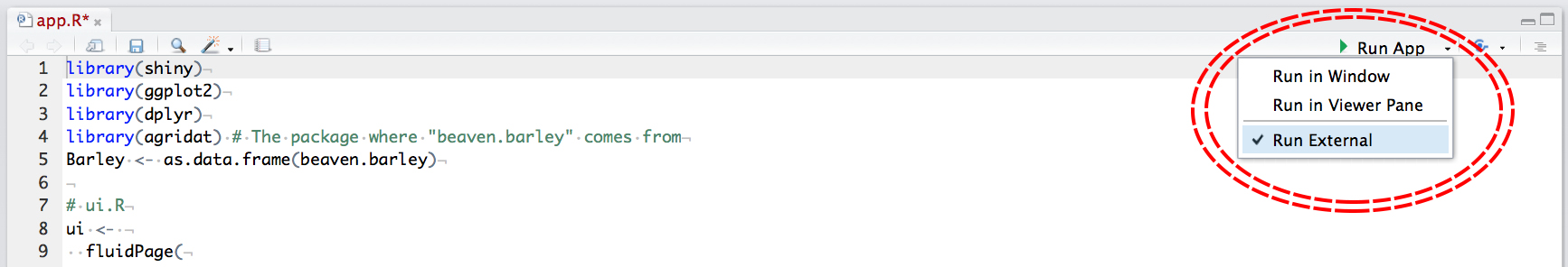
or use the keyboard shortcut Cmd + Opt + R (Mac), Ctrl + Alt + R (Windows).

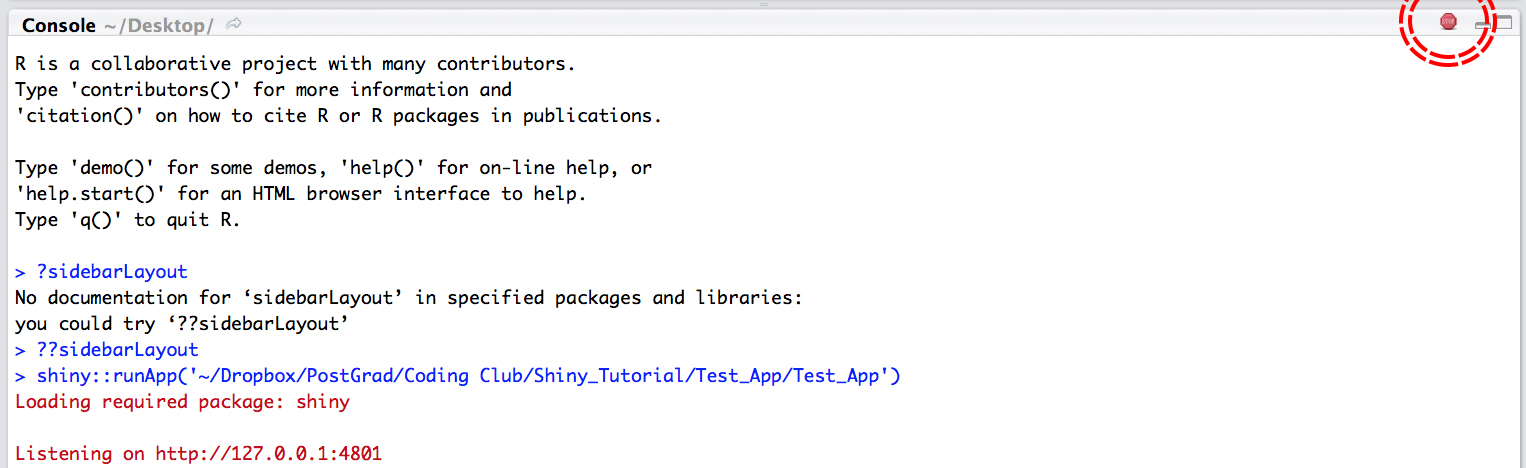
When a Shiny app is running from RStudio, the console cannot be used. To stop the app, click the Stop button in the top right of the console window or press the Esc key.

Output

A Shiny app without any outputs is useless. Outputs can be in the form of plots, tables, maps or text.

As per our example app, we’re going to be using ggplot() to create a histogram. For more information on creating plots in ggplot2, see our tutorials on basic data visualisation and customising ggplot graphs.

Outputs are created by placing code in the curly brackets ({}) in the server object:

server <- function(input, output) {
  output$plot <- renderPlot(ggplot(Barley, aes(x = yield)) +  # Create object called `output$plot` with a ggplot inside it
  geom_histogram(bins = 7,  # Add a histogram to the plot
    fill = "grey",  # Make the fill colour grey
    data = Barley,  # Use data from `Barley`
    colour = "black")  # Outline the bins in black
  )                                                       
}

Look at the code above for a couple of minutes to understand what is going on, then add it to your own app.R in the appropriate place.

Basically, we are creating an object called output$plot and using renderPlot() to wrap a ggplot() command.

Reactive output

The histogram is great, but not particularly interactive. We need to link our input widgets to our output object.

We want to select individual genotypes to display in our histogram, which the user can select using the selectInput that we called genotype earlier. Use some base R wizardry, [] $ and ==, to select the data we want. Update server with the new reactive output arguments so it looks like the code below:

server <- function(input, output) {
  output$plot <- renderPlot(ggplot(Barley, aes(x = yield)) +
  geom_histogram(bins = 7,
      fill = "grey",
      data = Barley[Barley$gen == input$gen,],
      colour = "black")
  )                                                       
}

data = Barley[Barley$Genotype == input$gen,] tells geom_histogram() to only use data where the value in column gen is equal to (==) the value given by input$gen. Note the , after input$gen which indicates that we are selecting columns and that all the rows should be selected.

Next, we want to be able to change the colour of the histogram based on the value of the selectInput called colour. To do this, simply change fill = “grey” to fill = input$colour.

Next, we want to select the number of bins in the histogram using the sliderInput called bin. Simply change bins = 7 to bins = input$bin.

Finally, to create a table output showing some summary statistics of the selected genotype, create a new output object called output$table and use renderTable() to create a table generated using dplyr summarise(). See our tutorial on data manipulation for more information on dplyr. Update server with the output$table information so it looks like the code below:

server <- function(input, output) {
output$myhist <- renderPlot(ggplot(Barley, aes(x = yield)) + 
	geom_histogram(bins = input$bin, fill = input$col, group=input$gen, 
		data=Barley[Barley$gen == input$gen,],
  		colour = "black"))

output$mytext <- renderText(input$text)

output$mytable <- renderTable(Barley %>%
filter(gen == input$gen) %>%
summarise("Mean" = mean(yield), 
  	"Median" = median(yield),
  	"STDEV" = sd(yield), 
  	"Min" = min(yield),
  	"Max" = max(yield)))
}

Displaying output

To make the outputs appear on your app in the mainPanel, they need to be added to the ui object inside mainPanel() like so:

ui <- 
  fluidPage(
    titlePanel("Barley Yield"),
    sidebarLayout(
      position = "right",
      sidebarPanel(h3("Inputs for histogram"), 
                   selectInput("gen", "1. Select genotype", choices = c("A" = "a","B" = "b","C" = "c","D" = "d","E" = "e","F" = "f","G" = "g","H" = "h"), selected = "a"),
                   br(),
                   selectInput("col", "2. Select histogram colour", choices = c("blue","green","red","purple","grey"), selected = "grey"),
                   br(),
                   sliderInput("bin", "3. Select number of histogram bins", min=1, max=25, value= c(10)),
                   br(),
                   textInput("text", "4. Enter some text to be displayed", "")),
                   mainPanel(
                             plotOutput("myhist"),
                             tableOutput("mytable"),
                             textOutput("mytext")
                             )
      )
    )

Take this chance to preview your app again by clicking Run in RStudio.

Additional elements

HTML

To make your app look more pretty, you can add HTML tags like in a normal HTML webpage. Below is a table of basic HTML tags, their Shiny equivalent and a description of what they do:

A list of all HTML tags can be found using:

shiny::tags

Some tags may conflict with other functions and so you should always state the source the function comes from by using tags$, e.g.:

tags$div()

Tags can be stacked to apply many arguments to the same object/text, just as in HTML:

tags$div(style="color:red",
  tags$p("Visit us at:"),
  tags$a(href = "https://ourcodingclub.github.io", "Coding Club")
  )

This creates a block of text that is coloured red (style="color:red"), within that block there is a paragraph of text (tags$p("Visit us at?:")) and a link (tags$a(href = "http://ourcodingglub.github.io", "Coding Club")).

Add the code above to your Shiny app in mainPanel() and see what happens!

For more information on the arguments that can be included in popular Shiny HTML tags, RStudio have a nice wiki at [[https://shiny.rstudio.com/articles/tag-glossary.html]].

5. Exporting a finished app

As a Github repository

It is easy to send a Shiny app to somebody else who also has RStudio. The easiest way is to send app.R alongside any data and other resources in a zip file to be unzipped by the recipient and run through R.

If you want to quickly share the app over the internet we recommend using Github to host the file.

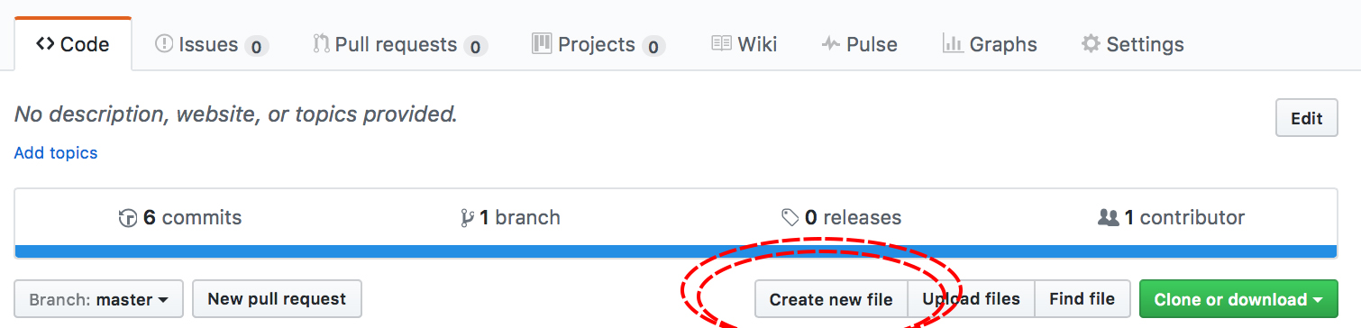
Go to Github, sign in with your account details, create a repository and upload everything from your app folder, including any Data and www folders.

Remember to add a file called README.md using Create new file in your new app repository, where you can write a quick explanation of the content of your app. .md files can use markdown syntax to create headers, sections, links etc.. See our tutorial on markdown and reproducible research for more markdown tips:

To send the app to another person, give them your Github username and the name of the app repo and ask them to run runGithub() in R, like this:

runGitHub(repo = "repo_name", username = "user_name")

Alternatively, if your recipient doesn’t know how Github works, upload your app folder as a .zip file to Github or any other file-hosting service and they can use runUrl() if you give them the url of the zipfile:

runUrl("https://github.com/rstudio/shiny_example/archive/master.zip")

To learn more about Github, check out our tutorial on Git and Github.

As a shinyapps.io app

You can also host Shiny apps on www.shinyapps.io, a webhosting platform run by RStudio that is especially built for Shiny apps. Go to their website and sign up using whatever method you choose, then go to www.shinyapps.io/admin/#/tokens, click Show secret and copy the rsconnect account info:

Then open up an R session and run the copied material to link shinyapps.io with R Studio.

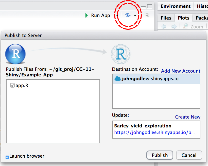
To upload your app, open your app.R and click the publish button. Select a name for your app (no spaces) and click Publish.

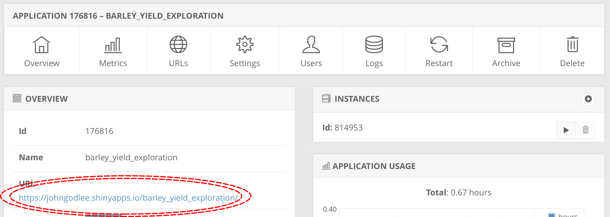
The app can then be used by anyone with the URL for that app, which can be found by going to shinyapps.io and opening the app info from the dashboard:

To embed an app that is hosted by shinyapps.io, in your own website you can put it in an iframe, replacing the URL with your own app URL and altering the style arguments to your own desire:

<iframe src="https://johngodlee.shinyapps.io/barley_yield_exploration/" style="border:none;width:1000px;height:500px;"></iframe>

6. Challenge yourself to create a Shiny app

Now that you have the skills to create a Shiny app, try to create an app of your own and publish it to your shinyapps.io profile. Your app could use your own data if you have some, or one of the many datasets that come bundled with R. If you need more inspiration, have a look through the Shiny app gallery.

Doing this tutorial as part of our Data Science for Ecologists and Environmental Scientists online course?

This tutorial is part of the Stats from Scratch stream from our online course. Go to the stream page to find out about the other tutorials part of this stream!

If you have already signed up for our course and you are ready to take the quiz, go to our quiz centre. Note that you need to sign up first before you can take the quiz. If you haven't heard about the course before and want to learn more about it, check out the course page.

Launch Quiz Centre