Created by Gabriela K Hajduk - last updated 9th February 2022 by Elise Gallois

This workshop is aimed at people new to mixed modeling and as such, it doesn’t cover all the nuances of mixed models, but hopefully serves as a starting point when it comes to both the concepts and the code syntax in R. There are no equations used to keep it beginner friendly.

Acknowledgements: First of all, thanks where thanks are due. This tutorial has been built on the tutorial written by Liam Bailey, who has been kind enough to let me use chunks of his script, as well as some of the data. Having this backbone of code made my life much, much easier, so thanks Liam, you are a star! The seemingly excessive waffling is mine.

If you are familiar with linear models, aware of their shortcomings and happy with their fitting, then you should be able to very quickly get through the first five sections below. Beginners might want to spend multiple sessions on this tutorial to take it all in.

Similarly, you will find quite a bit of explanatory text: you might choose to just skim it for now and go through the “coding bits” of the tutorial. But it will be here to help you along when you start using mixed models with your own data and you need a bit more context.

Alternatively, you can grab the R script here and the data from here. I might update this tutorial in the future and if I do, the latest version will be on my website.

Tutorial sections:

1. What is mixed effects modelling and why does it matter?
2. Explore the data
3. Fit all data in one analysis
4. Run multiple analyses
5. Modify the current model
6. Mixed effects models
   • Fixed and Random effects
   • Let’s fit our first mixed model
   • Types of random effects
     • Crossed random effects
     • Nested random effects
     • Implicit vs. explicit nesting
   • Our second mixed model
   • Introducing random slopes
   • Presenting your model results
     • Plotting model predictions
     • Tables
     • Further processing
   • EXTRA: P-values and model selection
     • Fixed effects structure
     • Random effects structure
     • The entire model selection
7. THE END

1. What is mixed effects modelling and why does it matter?

Ecological and biological data are often complex and messy. We can have different grouping factors like populations, species, sites where we collect the data, etc. Sample sizes might leave something to be desired too, especially if we are trying to fit complicated models with many parameters. On top of that, our data points might not be truly independent. For instance, we might be using quadrats within our sites to collect the data (and so there is structure to our data: quadrats are nested within the sites).

This is why mixed models were developed, to deal with such messy data and to allow us to use all our data, even when we have low sample sizes, structured data and many covariates to fit. Oh, and on top of all that, mixed models allow us to save degrees of freedom compared to running standard linear models! Sounds good, doesn’t it?

We will cover only linear mixed models here, but if you are trying to “extend” your linear model, fear not: there are generalised linear mixed effects models out there, too.

2. Explore the data

We are going to focus on a fictional study system, dragons, so that we don’t have to get too distracted with the specifics of this example. Imagine that we decided to train dragons and so we went out into the mountains and collected data on dragon intelligence (testScore) as a prerequisite. We sampled individuals with a range of body lengths across three sites in eight different mountain ranges. Start by loading the data and having a look at them.

load("dragons.RData")
head(dragons)

Let’s say we want to know how the body length of the dragons affects their test scores.

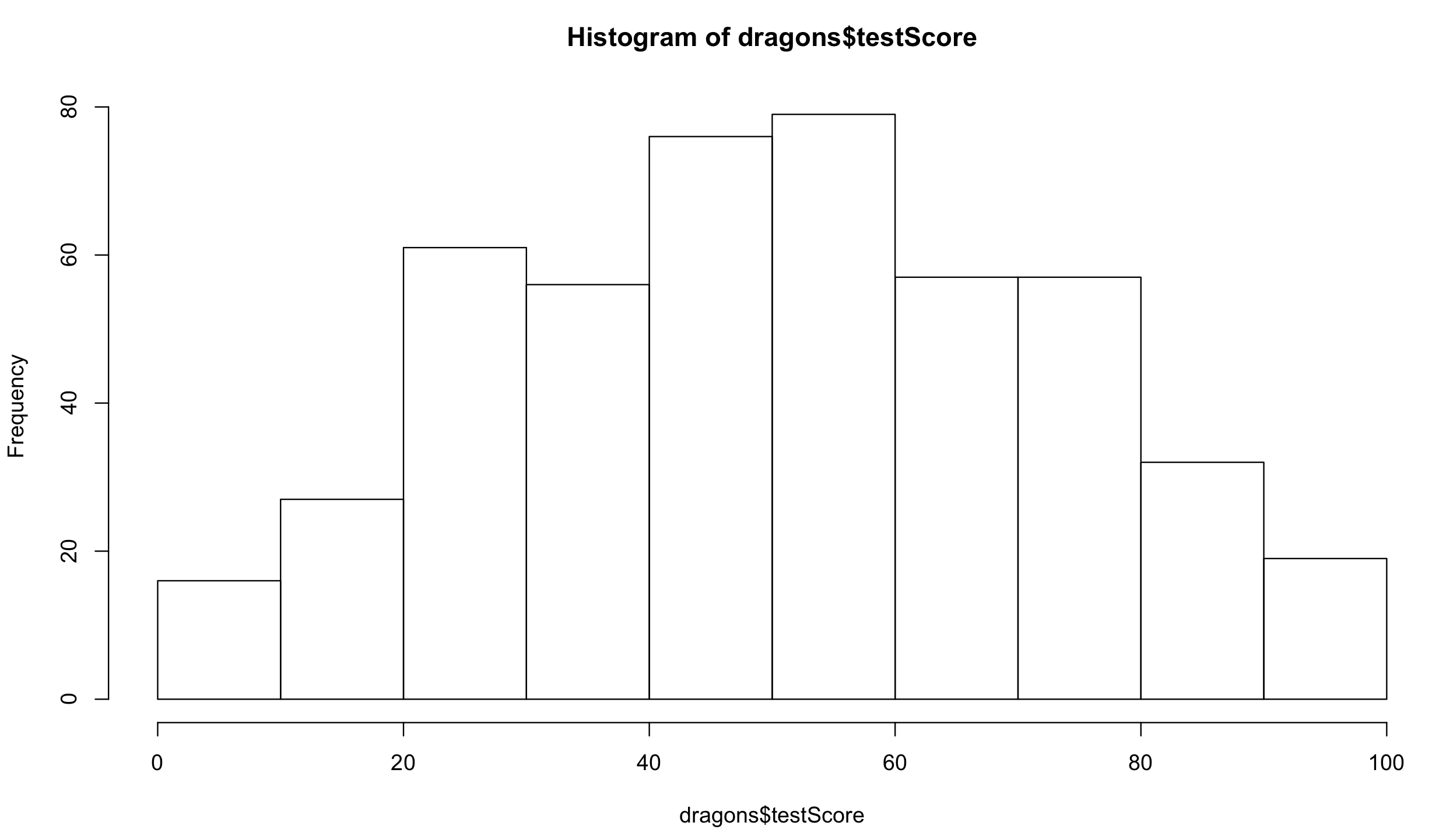
You don’t need to worry about the distribution of your explanatory variables. Have a look at the distribution of the response variable:

hist(dragons$testScore)  # seems close to a normal distribution - good!

It is good practice to standardise your explanatory variables before proceeding so that they have a mean of zero (“centering”) and standard deviation of one (“scaling”). It ensures that the estimated coefficients are all on the same scale, making it easier to compare effect sizes. You can use scale() to do that:

dragons$bodyLength2 <- scale(dragons$bodyLength, center = TRUE, scale = TRUE)

scale() centers the data (the column mean is subtracted from the values in the column) and then scales it (the centered column values are divided by the column’s standard deviation).

Back to our question: is the test score affected by body length?

3. Fit all data in one analysis

One way to analyse this data would be to fit a linear model to all our data, ignoring the sites and the mountain ranges for now.

Fit the model with testScore as the response and bodyLength2 as the predictor and have a look at the output:

basic.lm <- lm(testScore ~ bodyLength2, data = dragons)
summary(basic.lm)

Let’s plot the data with ggplot2.

library(tidyverse)  # load the package containing both ggplot2 and dplyr

(prelim_plot <- ggplot(dragons, aes(x = bodyLength, y = testScore)) +
  geom_point() +
  geom_smooth(method = "lm"))
  

Note that putting your entire ggplot code in brackets () creates the graph and then shows it in the plot viewer. If you don’t have the brackets, you’ve only created the object, but haven’t visualised it. You would then have to call the object such that it will be displayed by just typing prelim_plot after you’ve created the “prelim_plot” object.

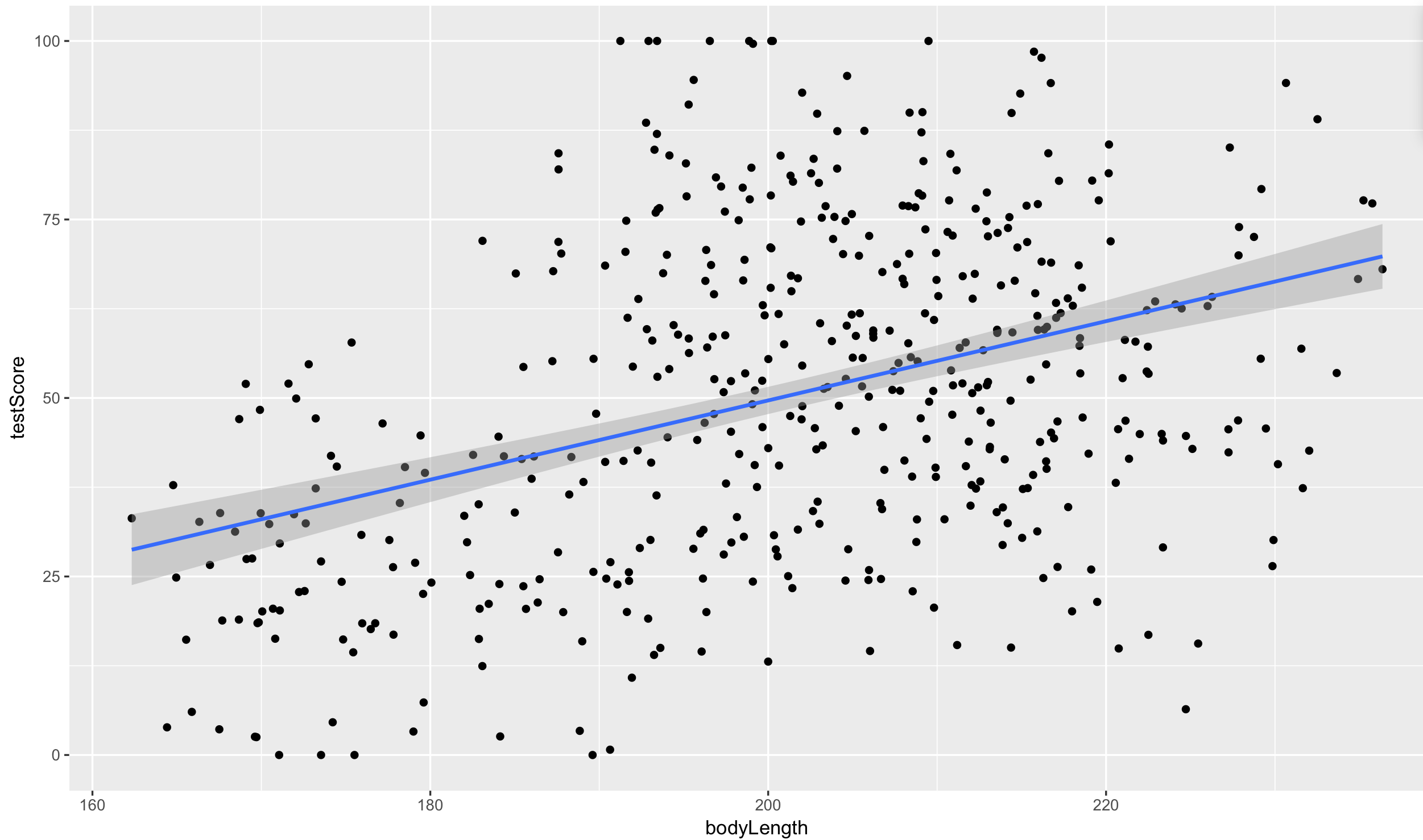
Okay, so both from the linear model and from the plot, it seems like bigger dragons do better in our intelligence test. That seems a bit odd: size shouldn’t really affect the test scores.

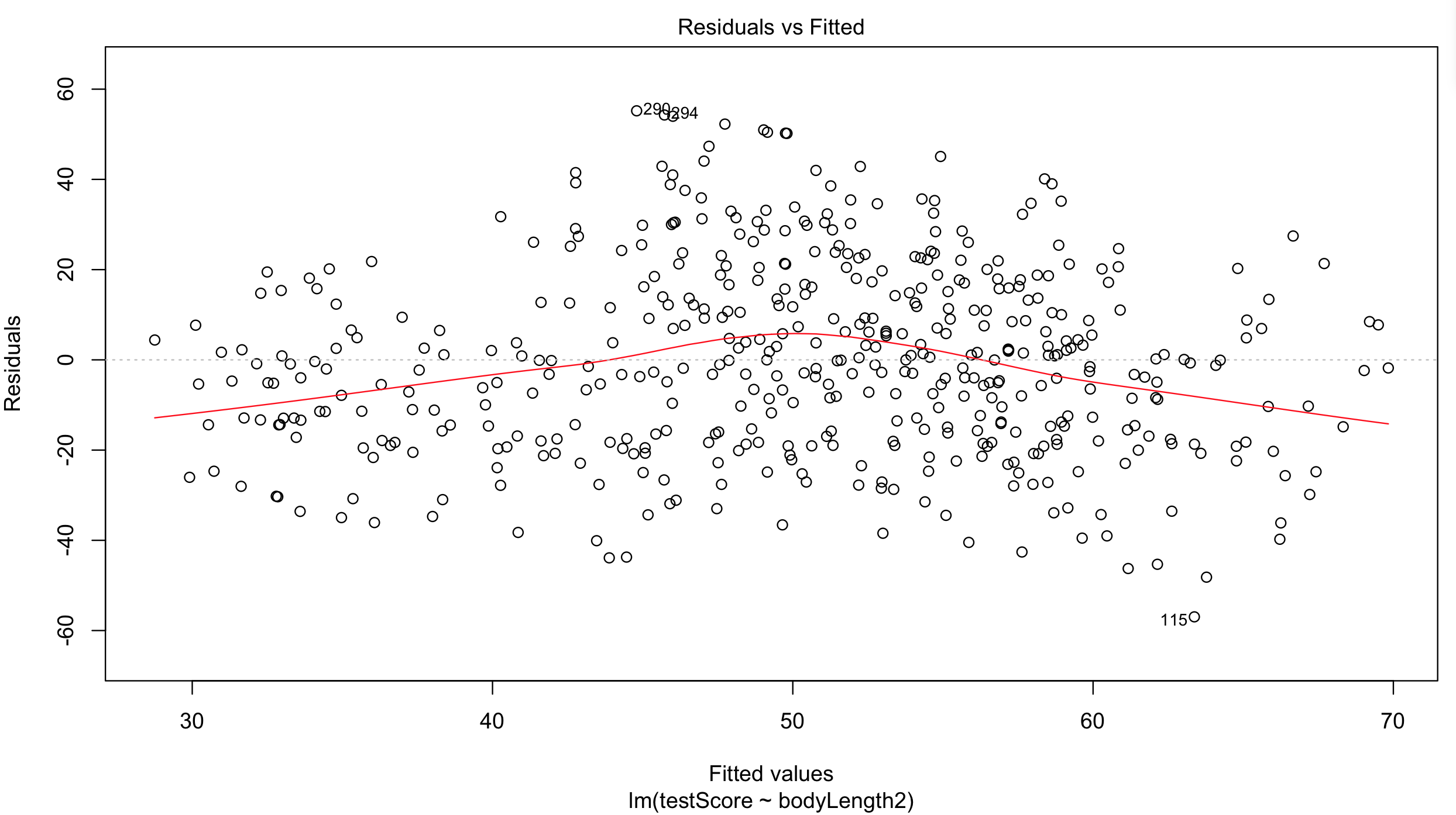
But… are the assumptions met?

Plot the residuals: the red line should be nearly flat, like the dashed grey line:

plot(basic.lm, which = 1)  # not perfect... 
## but since this is a fictional example we will go with it
## for your own data be careful:
## the bigger the sample size, the less of a trend you'd expect to see

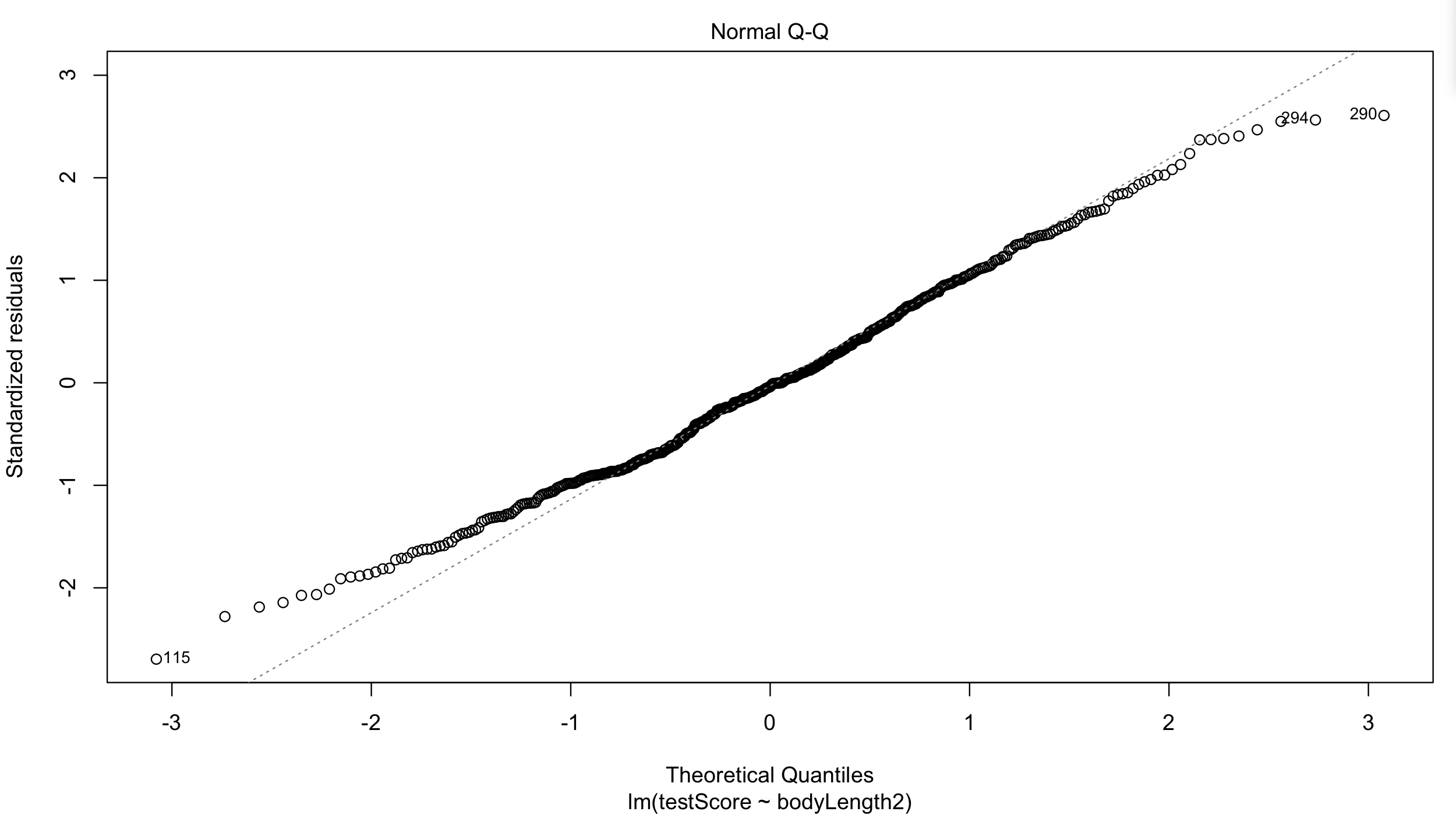
Have a quick look at the qqplot too: points should ideally fall onto the diagonal dashed line:

plot(basic.lm, which = 2)  # a bit off at the extremes, but that's often the case; again doesn't look too bad

However, what about observation independence? Are our data independent?

We collected multiple samples from eight mountain ranges. It’s perfectly plausible that the data from within each mountain range are more similar to each other than the data from different mountain ranges: they are correlated.

Have a look at the data to see if above is true:

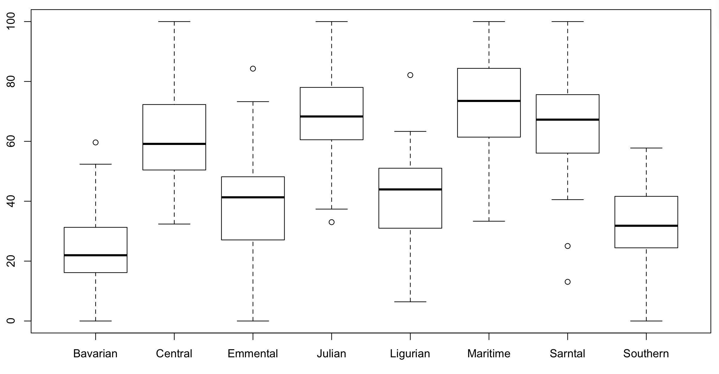
boxplot(testScore ~ mountainRange, data = dragons)  # certainly looks like something is going on here

We could also plot it and colour points by mountain range:

(colour_plot <- ggplot(dragons, aes(x = bodyLength, y = testScore, colour = mountainRange)) +
  geom_point(size = 2) +
  theme_classic() +
  theme(legend.position = "none"))

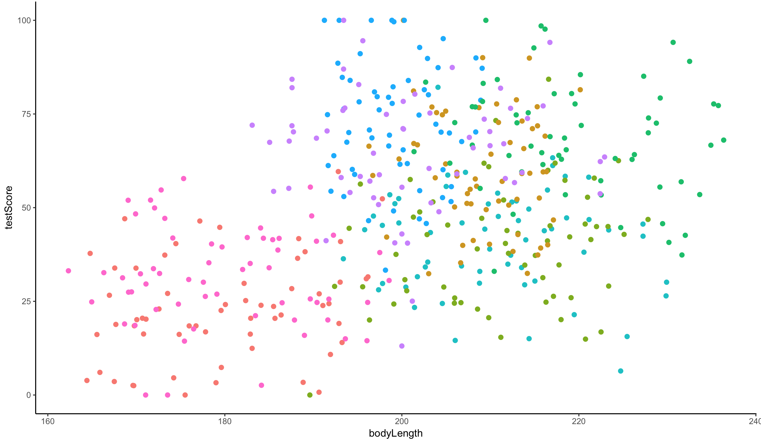
From the above plots, it looks like our mountain ranges vary both in the dragon body length AND in their test scores. This confirms that our observations from within each of the ranges aren’t independent. We can’t ignore that: as we’re starting to see, it could lead to a completely erroneous conclusion.

So what do we do?

4. Run multiple analyses

We could run many separate analyses and fit a regression for each of the mountain ranges.

Lets have a quick look at the data split by mountain range. We use the facet_wrap to do that:

(split_plot <- ggplot(aes(bodyLength, testScore), data = dragons) + 
  geom_point() + 
  facet_wrap(~ mountainRange) + # create a facet for each mountain range
  xlab("length") + 
  ylab("test score"))

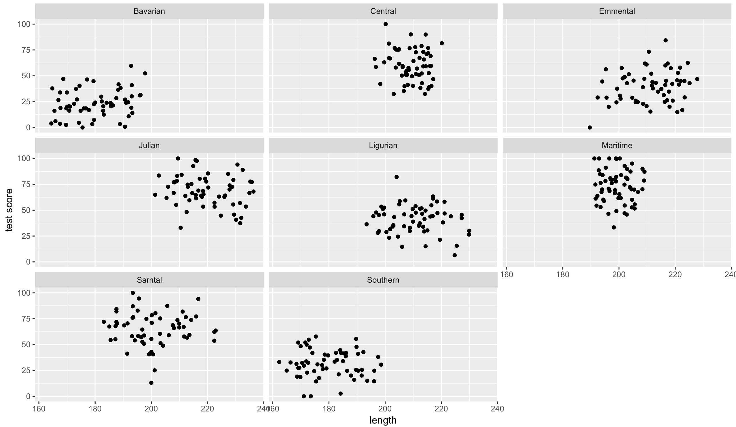
That’s eight analyses. Oh wait, we also have different sites in each mountain range, which similarly to mountain ranges aren’t independent… So we could run an analysis for each site in each range separately.

To do the above, we would have to estimate a slope and intercept parameter for each regression. That’s two parameters, three sites and eight mountain ranges, which means 48 parameter estimates (2 x 3 x 8 = 48)! Moreover, the sample size for each analysis would be only 20 (dragons per site).

This presents problems: not only are we hugely decreasing our sample size, but we are also increasing chances of a Type I Error (where you falsely reject the null hypothesis) by carrying out multiple comparisons. Not ideal!

5. Modify the current model

We want to use all the data, but account for the data coming from different mountain ranges (let’s put sites on hold for a second to make things simpler).

Add mountain range as a fixed effect to our basic.lm

mountain.lm <- lm(testScore ~ bodyLength2 + mountainRange, data = dragons)
summary(mountain.lm)

Now body length is not significant. But let’s think about what we are doing here for a second. The above model is estimating the difference in test scores between the mountain ranges - we can see all of them in the model output returned by summary(). But we are not interested in quantifying test scores for each specific mountain range: we just want to know whether body length affects test scores and we want to simply control for the variation coming from mountain ranges.

This is what we refer to as “random factors” and so we arrive at mixed effects models. Ta-daa!

6. Mixed effects models

A mixed model is a good choice here: it will allow us to use all the data we have (higher sample size) and account for the correlations between data coming from the sites and mountain ranges. We will also estimate fewer parameters and avoid problems with multiple comparisons that we would encounter while using separate regressions.

We are going to work in lme4, so load the package (or use install.packages if you don’t have lme4 on your computer).

library(lme4)

Fixed and random effects

Let’s talk a little about the difference between fixed and random effects first. It’s important to not that this difference has little to do with the variables themselves, and a lot to do with your research question! In many cases, the same variable could be considered either a random or a fixed effect (and sometimes even both at the same time!) so always refer to your questions and hypotheses to construct your models accordingly.

test <- 1 + 3

In our particular case, we are looking to control for the effects of mountain range. We haven’t sampled all the mountain ranges in the world (we have eight) so our data are just a sample of all the existing mountain ranges. We are not really interested in the effect of each specific mountain range on the test score: we hope our model would also be generalisable to dragons from other mountain ranges! However, we know that the test scores from within the ranges might be correlated so we want to control for that.

If we specifically chose eight particular mountain ranges a priori and we were interested in those ranges and wanted to make predictions about them, then mountain range would be fitted as a fixed effect.

In the end, the big questions are: what are you trying to do? What are you trying to make predictions about? What is just variation (a.k.a “noise”) that you need to control for?

Let’s fit our first mixed model

Alright! Still with me? We have a response variable, the test score and we are attempting to explain part of the variation in test score through fitting body length as a fixed effect. But the response variable has some residual variation (i.e. unexplained variation) associated with mountain ranges. By using random effects, we are modeling that unexplained variation through variance.

[Sidenote: If you are confused between variation and variance: variation is a generic word, similar to dispersion or variability; variance is a particular measure of variation; it quantifies the dispersion, if you wish.]

Note that our question changes slightly here: while we still want to know whether there is an association between dragon’s body length and the test score, we want to know if that association exists after controlling for the variation in mountain ranges.

We will fit the random effect using the syntax (1|variableName):

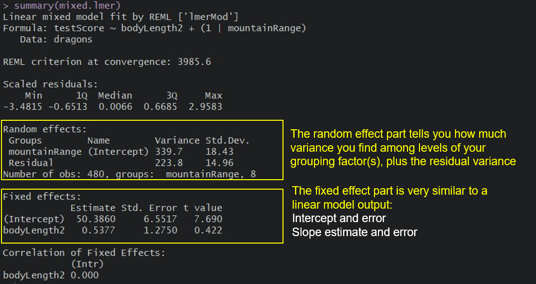
mixed.lmer <- lmer(testScore ~ bodyLength2 + (1|mountainRange), data = dragons)
summary(mixed.lmer)

Once we account for the mountain ranges, it’s obvious that dragon body length doesn’t actually explain the differences in the test scores. How is it obvious? I hear you say?

Take a look at the summary output: notice how the model estimate is smaller than its associated error? That means that the effect, or slope, cannot be distinguised from zero.

Keep in mind that the random effect of the mountain range is meant to capture all the influences of mountain ranges on dragon test scores - whether we observed those influences explicitly or not, whether those influences are big or small etc. It could be many, many teeny-tiny influences that, when combined, affect the test scores and that’s what we are hoping to control for.

We can see the variance for mountainRange = 339.7. Mountain ranges are clearly important: they explain a lot of variation. How do we know that? We can take the variance for the mountainRange and divide it by the total variance:

339.7/(339.7 + 223.8)  # ~60 %

So the differences between mountain ranges explain ~60% of the variance that’s “left over” after the variance explained by our fixed effects.

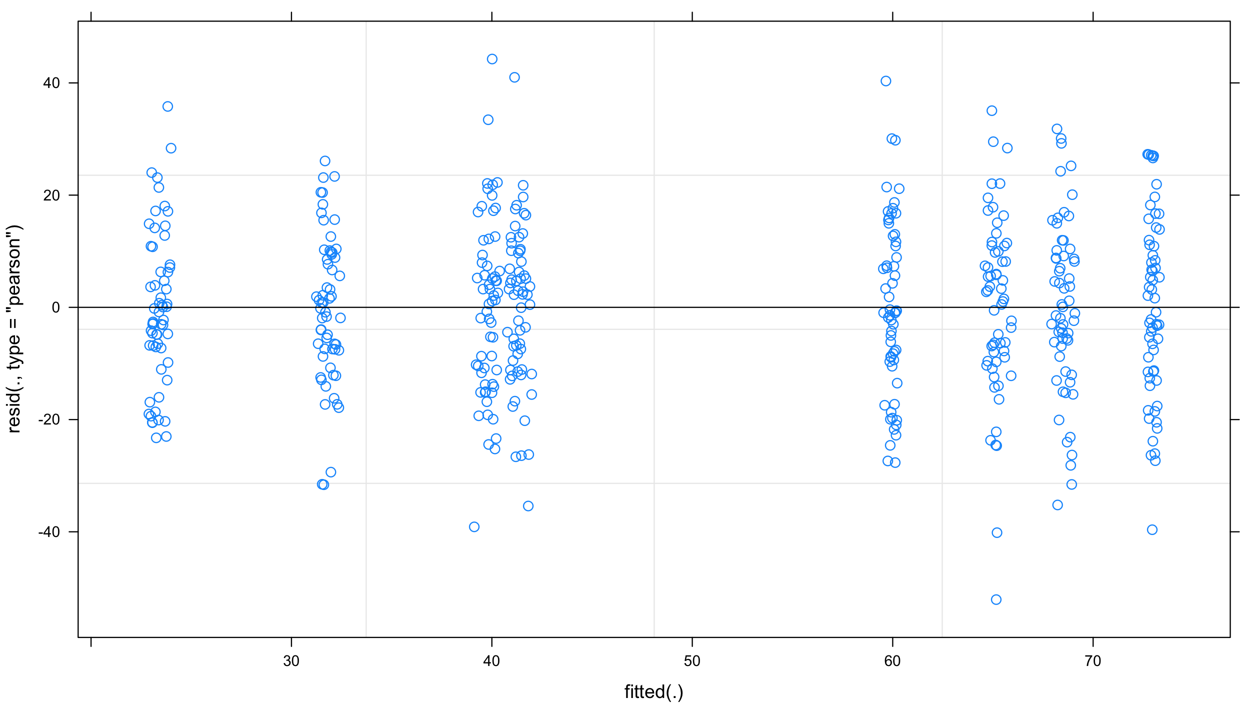
As always, it’s good practice to have a look at the plots to check our assumptions:

plot(mixed.lmer)  # looks alright, no patterns evident

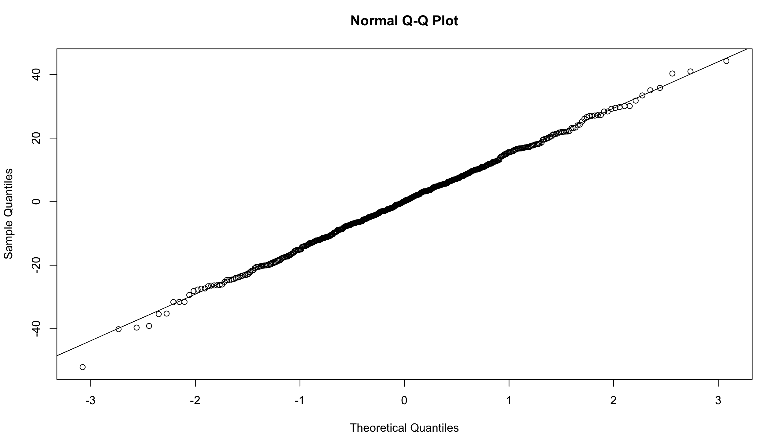
and qqplot:

qqnorm(resid(mixed.lmer))
qqline(resid(mixed.lmer))  # points fall nicely onto the line - good!

Types of random effects

Before we go any further, let’s review the syntax above and chat about crossed and nested random effects. It’s useful to get those clear in your head.

Reminder: a factor is just any categorical independent variable.

Above, we used (1|mountainRange) to fit our random effect. Whatever is on the right side of the | operator is a factor and referred to as a “grouping factor” for the term.

Random effects (factors) can be crossed or nested - it depends on the relationship between the variables. Let’s have a look.

Crossed random effects

Be careful with the nomenclature. There are “hierarchical linear models” (HLMs) or “multilevel models” out there, but while all HLMs are mixed models, not all mixed models are hierarchical. That’s because you can have crossed (or partially crossed) random factors that do not represent levels in a hierarchy.

Think for instance about our study where you monitor dragons (subject) across different mountain ranges (context) and imagine that we collect multiple observations per dragon by giving it the test multiple times (and risking pseudoreplication - but more on that later). Since our dragons can fly, it’s easy to imagine that we might observe the same dragon across different mountain ranges, but also that we might not see all the dragons visiting all of the mountain ranges. Therefore, we can potentially observe every dragon in every mountain range (crossed) or at least observe some dragons across some of the mountain ranges (partially crossed). We would then fit the identity of the dragon and mountain range as (partially) crossed random effects.

Let’s repeat with another example: an effect is (fully) crossed when all the subjects have experienced all the levels of that effect. For instance, if you had a fertilisation experiment on seedlings growing in a seasonal forest and took repeated measurements over time (say 3 years) in each season, you may want to have a crossed factor called season (Summer1, Autumn1, Winter1, Spring1, Summer2, …, Spring3), i.e. a factor for each season of each year. This grouping factor would account for the fact that all plants in the experiment, regardless of the fixed (treatment) effect (i.e. fertilised or not), may have experienced a very hot summer in the second year, or a very rainy spring in the third year, and those conditions could cause interference in the expected patterns. You don’t even need to have associated climate data to account for it! You just know that all observations from spring 3 may be more similar to each other because they experienced the same environmental quirks rather than because they’re responding to your treatment.

If this sounds confusing, not to worry - lme4 handles partially and fully crossed factors well. Now, let’s look at nested random effects and how to specify them.

Nested random effects

If you’re not sure what nested random effects are, think of those Russian nesting dolls. We’ve already hinted that we call these models hierarchical: there’s often an element of scale, or sampling stratification in there.

Take our fertilisation experiment example again; let’s say you have 50 seedlings in each bed, with 10 control and 10 experimental beds. That’s 1000 seedlings altogether. And let’s say you went out collecting once in each season in each of the 3 years. On each plant, you measure the length of 5 leaves. That’s….(lots of maths)…5 leaves x 50 plants x 20 beds x 4 seasons x 3 years….. 60 000 measurements!

But if you were to run the analysis using a simple linear regression, eg. leafLength ~ treatment , you would be committing the crime (!!) of pseudoreplication, or massively increasing your sampling size by using non-independent data. With a sample size of 60,000 you would almost certainly get a “significant” effect of treatment which may have no ecological meaning at all. And it violates the assumption of independance of observations that is central to linear regression.

This is where our nesting dolls come in; leaves within a plant and plants within a bed may be more similar to each other (e.g. for genetic and environmental reasons, respectively). You could therefore add a random effect structure that accounts for this nesting:

leafLength ~ treatment + (1|Bed/Plant/Leaf)

This way, the model will account for non independence in the data: the same leaves have been sampled repeatedly, multiple leaves were measured on an individual, and plants are grouped into beds which may receive different amounts of sun, etc.

What about the crossed effects we mentioned earlier? If all the leaves have been measured in all seasons, then your model would become something like:

leafLength ~ treatment + (1|Bed/Plant/Leaf) + (1|Season)

Phew!

head(dragons)  # we have site and mountainRange
str(dragons)  # we took samples from three sites per mountain range and eight mountain ranges in total

dragons <- within(dragons, sample <- factor(mountainRange:site))

Our second mixed model

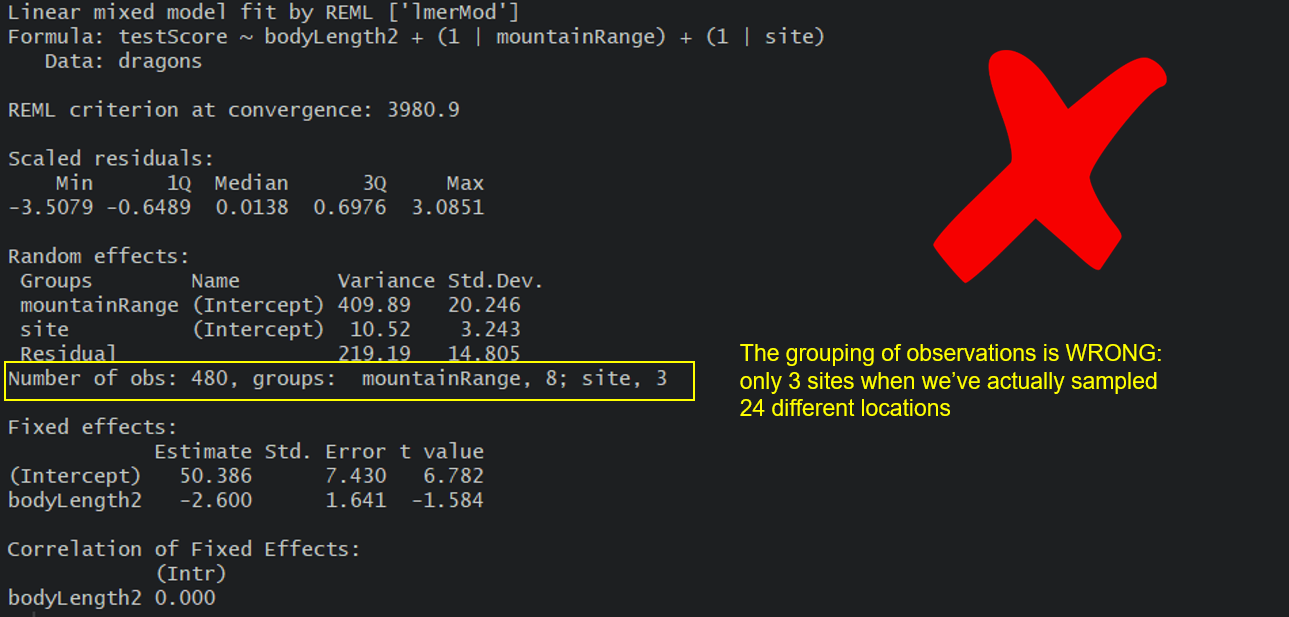
Based on the above, using following specification would be **wrong**, as it would imply that there are only three sites with observations at each of the 8 mountain ranges (crossed):

mixed.WRONG <- lmer(testScore ~ bodyLength2 + (1|mountainRange) + (1|site), data = dragons)  # treats the two random effects as if they are crossed
summary(mixed.WRONG)

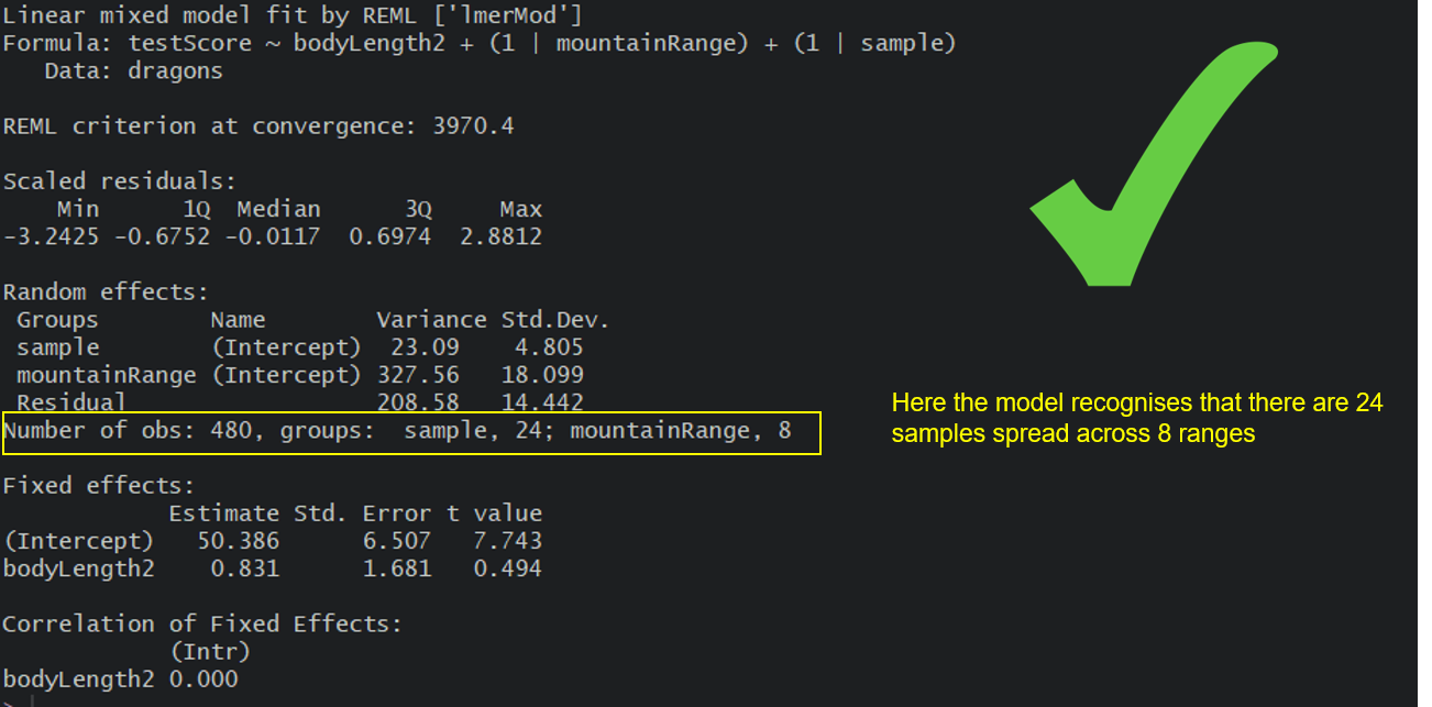
But we can go ahead and fit a new model, one that takes into account both the differences between the mountain ranges, as well as the differences between the sites within those mountain ranges by using our sample variable.

Our question gets adjusted slightly again: Is there an association between body length and intelligence in dragons after controlling for variation in mountain ranges and sites within mountain ranges?

mixed.lmer2 <- lmer(testScore ~ bodyLength2 + (1|mountainRange) + (1|sample), data = dragons)  # the syntax stays the same, but now the nesting is taken into account
summary(mixed.lmer2)

Here, we are trying to account for all the mountain-range-level and all the site-level influences and we are hoping that our random effects have soaked up all these influences so we can control for them in the model.

For the record, you could also use the below syntax, and you will often come across it if you read more about mixed models:

(1|mountainRange/site) or even (1|mountainRange) + (1|mountainRange:site)

However, it is advisable to set out your variables properly and make sure nesting is stated explicitly within them, that way you don’t have to remember to specify the nesting.

Let’s plot this again - visualising what’s going on is always helpful. You should be able to see eight mountain ranges with three sites (different colour points) within them, with a line fitted through each site.

(mm_plot <- ggplot(dragons, aes(x = bodyLength, y = testScore, colour = site)) +
      facet_wrap(~mountainRange, nrow=2) +   # a panel for each mountain range
      geom_point(alpha = 0.5) +
      theme_classic() +
      geom_line(data = cbind(dragons, pred = predict(mixed.lmer2)), aes(y = pred), size = 1) +  # adding predicted line from mixed model 
      theme(legend.position = "none",
            panel.spacing = unit(2, "lines"))  # adding space between panels
)

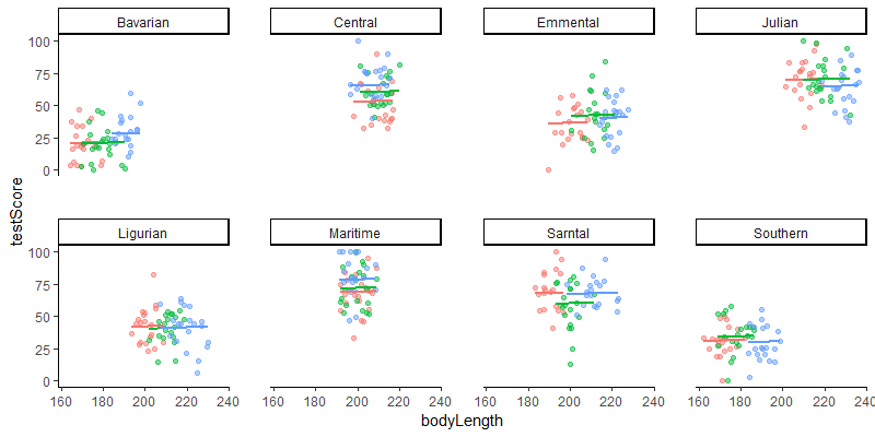
Introducing random slopes

You might have noticed that all the lines on the above figure are parallel: that’s because so far, we have only fitted random-intercept models. A random-intercept model allows the intercept to vary for each level of the random effects, but keeps the slope constant among them. So in our case, using this model means that we expect dragons in all mountain ranges to exhibit the same relationship between body length and intelligence (fixed slope), although we acknowledge that some populations may be smarter or dumber to begin with (random intercept).

You can find an excellent visualisation of random intercepts and slopes at this website

Now, in the life sciences, we perhaps more often assume that not all populations would show the exact same relationship, for instance if your study sites/populations are very far apart and have some relatively important environmental, genetic, etc differences. Therefore, we often want to fit a random-slope and random-intercept model. Maybe the dragons in a very cold vs a very warm mountain range have evolved different body forms for heat conservation and may therefore be smart even if they’re smaller than average.

We only need to make one change to our model to allow for random slopes as well as intercept, and that’s adding the fixed variable into the random effect brackets:

mixed.ranslope <- lmer(testScore ~ bodyLength2 + (1 + bodyLength2|mountainRange/site), data = dragons) 

summary(mixed.ranslope)

Here, we’re saying, let’s model the intelligence of dragons as a function of body length, knowing that populations have different intelligence baselines and that the relationship may vary among populations.

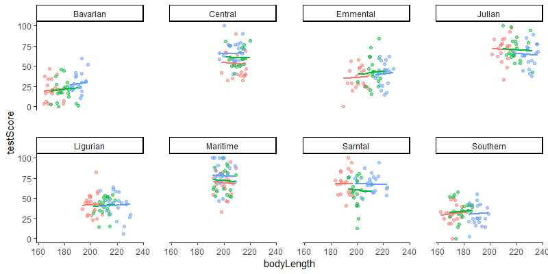
Let’s see that with a quick plot (we’ll plot predictions in more detail in the next section). Notice how the slopes for the different sites and mountain ranges are not parallel anymore?

### plot
(mm_plot <- ggplot(dragons, aes(x = bodyLength, y = testScore, colour = site)) +
      facet_wrap(~mountainRange, nrow=2) +   # a panel for each mountain range
      geom_point(alpha = 0.5) +
      theme_classic() +
      geom_line(data = cbind(dragons, pred = predict(mixed.ranslope)), aes(y = pred), size = 1) +  # adding predicted line from mixed model 
      theme(legend.position = "none",
            panel.spacing = unit(2, "lines"))  # adding space between panels
)

Well done for getting here! You have now fitted random-intercept and random-slopes, random-intercept mixed models and you know how to account for hierarchical and crossed random effects. You saw that failing to account for the correlation in data might lead to misleading results - it seemed that body length affected the test score until we accounted for the variation coming from mountain ranges. We can see now that body length doesn’t influence the test scores - great! We can pick smaller dragons for any future training - smaller ones should be more manageable!

If you are particularly keen, the next section gives you a few options when it comes to presenting your model results and in the last “extra” section you can learn about the model selection conundrum. There is just a little bit more code there to get through if you fancy those.

Presenting your model results

Once you get your model, you have to present it in a nicer form.

Plotting model predictions

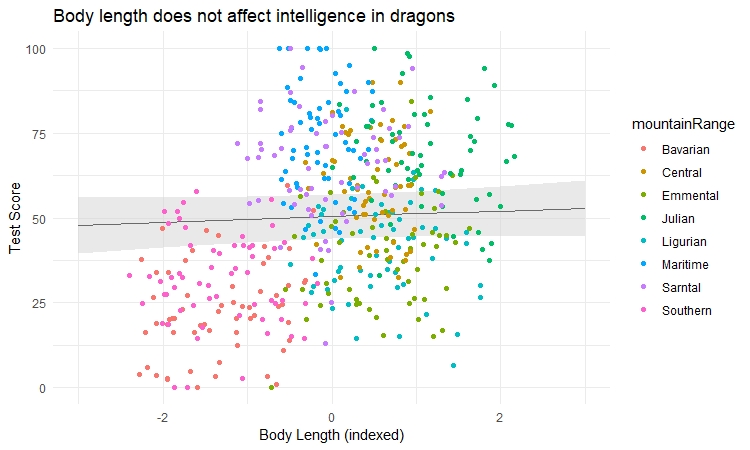
Often you will want to visualise your model as a regression line with some error around it, just like you would a simple linear model. However, ggplot2 stats options are not designed to estimate mixed-effect model objects correctly, so we will use the ggeffects package to help us draw the plots.

library(ggeffects)  # install the package first if you haven't already, then load it

# Extract the prediction data frame
pred.mm <- ggpredict(mixed.lmer2, terms = c("bodyLength2"))  # this gives overall predictions for the model

# Plot the predictions 

(ggplot(pred.mm) + 
   geom_line(aes(x = x, y = predicted)) +          # slope
   geom_ribbon(aes(x = x, ymin = predicted - std.error, ymax = predicted + std.error), 
               fill = "lightgrey", alpha = 0.5) +  # error band
   geom_point(data = dragons,                      # adding the raw data (scaled values)
              aes(x = bodyLength2, y = testScore, colour = mountainRange)) + 
   labs(x = "Body Length (indexed)", y = "Test Score", 
        title = "Body length does not affect intelligence in dragons") + 
   theme_minimal()
)

What if you want to visualise how the relationships vary according to different levels of random effects? You can specify type = "re" (for “random effects”) in the ggpredict() function, and add the random effect name to the terms argument.

We also demonstrate a way to plot the graph quicker with the plot() function of ggEffects:

ggpredict(mixed.lmer2, terms = c("bodyLength2", "mountainRange"), type = "re") %>% 
   plot() +
   labs(x = "Body Length", y = "Test Score", title = "Effect of body size on intelligence in dragons") + 
   theme_minimal()

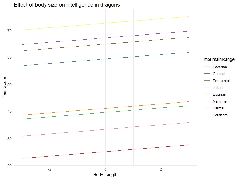
You can clearly see the random intercepts and fixed slopes from this graph. When assessing the quality of your model, it’s always a good idea to look at the raw data, the summary output, and the predictions all together to make sure you understand what is going on (and that you have specified the model correctly).

Another way to visualise mixed model results, if you are interested in showing the variation among levels of your random effects, is to plot the departure from the overall model estimate for intercepts - and slopes, if you have a random slope model:

library(sjPlot)

# Visualise random effects 
(re.effects <- plot_model(mixed.ranslope, type = "re", show.values = TRUE))

# show summary
summary(mixed.ranslope)

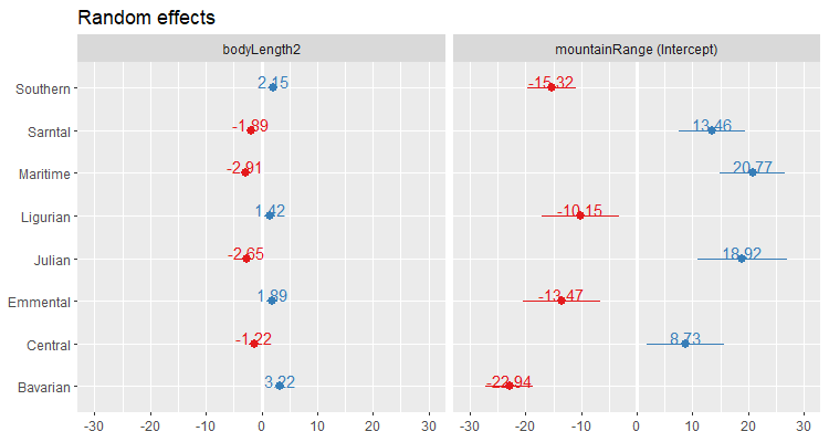
Careful here! The values you see are NOT actual values, but rather the difference between the general intercept or slope value found in your model summary and the estimate for this specific level of random effect. For instance, the relationship for dragons in the Maritime mountain range would have a slope of (-2.91 + 0.67) = -2.24 and an intercept of (20.77 + 51.43) = 72.20.

If you are looking for more ways to create plots of your results, check out dotwhisker and this tutorial.

Tables

For lme4, if you are looking for a table, I’d recommend that you have a look at the stargazer package.

library(stargazer)

stargazeris very nicely annotated and there are lots of resources (e.g. this) out there and a great cheat sheet so I won’t go into too much detail, as I’m confident you will find everything you need.

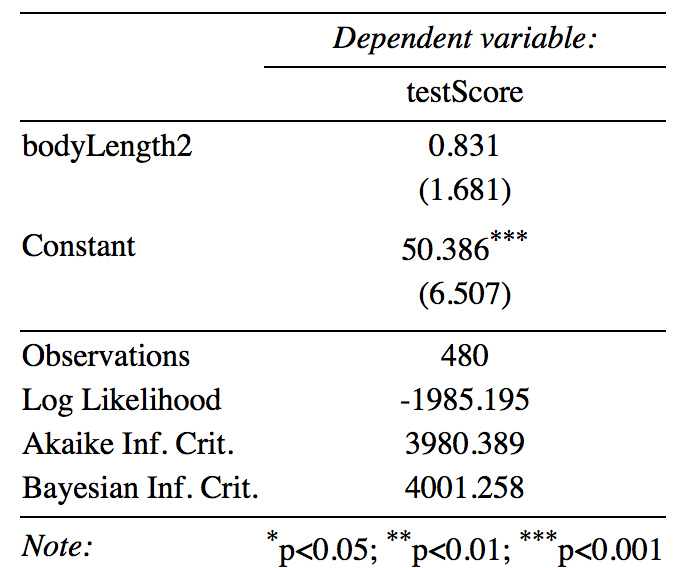
Here is a quick example - simply plug in your model name, in this case mixed.lmer2 into the stargazer function. I set type to "text" so that you can see the table in your console. I usually tweak the table like this until I’m happy with it and then export it using type = "latex", but "html" might be more useful for you if you are not a LaTeX user.

If you are keen, explore this table a little further - what would you change? What would you get rid off?

stargazer(mixed.lmer2, type = "text",
          digits = 3,
          star.cutoffs = c(0.05, 0.01, 0.001),
          digit.separator = "")

Further processing

If you’d like to be able to do more with your model results, for instance process them further, collate model results from multiple models or plot, them have a look at the broom package. This tutorial is a great start.

EXTRA: P-values and model selection

Please be very, very careful when it comes to model selection. Focus on your question, don’t just plug in and drop variables from a model haphazardly until you make something “significant”. Always choose variables based on biology/ecology: I might use model selection to check a couple of non-focal parameters, but I keep the “core” of the model untouched in most cases. Define your goals and questions and focus on that. Also, don’t just put all possible variables in (i.e. don’t overfit). Remember that as a rule of thumb, you need 10 times more data than parameters you are trying to estimate.

For more info on overfitting check out this tutorial.

Fixed effects structure

Before we start, again: think twice before trusting model selection!

Most of you are probably going to be predominantly interested in your fixed effects, so let’s start here. lme4 doesn’t spit out p-values for the parameters by default. This is a conscious choice made by the authors of the package, as there are many problems with p-values (I’m sure you are aware of the debates!).

You will inevitably look for a way to assess your model though so here are a few solutions on how to go about hypothesis testing in linear mixed models (LMMs):

From worst to best:

• Wald Z-tests
• Wald t-tests (but LMMs need to be balanced and nested)
• Likelihood ratio tests (via anova() or drop1())
• MCMC or parametric bootstrap confidence intervals

See this link for more information and further reading.

I think that MCMC and bootstrapping are a bit out of our reach for this workshop so let’s have a quick go at likelihood ratio tests using anova(). With large sample sizes, p-values based on the likelihood ratio are generally considered okay. NOTE: With small sample sizes, you might want to look into deriving p-values using the Kenward-Roger or Satterthwaite approximations (for REML models). Check out the pbkrtest package.

Fit the models, a full model and a reduced model in which we dropped our fixed effect (bodyLength2):

full.lmer <- lmer(testScore ~ bodyLength2 + (1|mountainRange) + (1|sample), 
				  data = dragons, REML = FALSE)
reduced.lmer <- lmer(testScore ~ 1 + (1|mountainRange) + (1|sample), 
					     data = dragons, REML = FALSE)

Compare them:

anova(reduced.lmer, full.lmer)  # the two models are not significantly different

Notice that we have fitted our models with REML = FALSE.

REML stands for restricted (or “residual”) maximum likelihood and it is the default parameter estimation criterion for linear mixed models. As you probably guessed, ML stands for maximum likelihood - you can set REML = FALSE in your call to lmer to use ML estimates. However, ML estimates are known to be biased and with REML being usually less biased, REML estimates of variance components are generally preferred. This is why in our previous models we skipped setting REML - we just left it as default (i.e. REML = TRUE).

REML assumes that the fixed effects structure is correct. You should use maximum likelihood when comparing models with different fixed effects, as ML doesn’t rely on the coefficients of the fixed effects - and that’s why we are refitting our full and reduced models above with the addition of REML = FALSE in the call.

Even though you use ML to compare models, you should report parameter estimates from your final “best” REML model, as ML may underestimate variance of the random effects.

NOTE 2: Models can also be compared using the AICc function from the AICcmodavg package. The Akaike Information Criterion (AIC) is a measure of model quality. AICc corrects for bias created by small sample size when estimating AIC. Generally, if models are within 2 AICc units of each other they are very similar. Within 5 units they are quite similar, over 10 units difference and you can probably be happy with the model with lower AICc. As with p-values though, there is no “hard line” that’s always correct.

NOTE 3: There isn’t really an agreed upon way of dealing with the variance from the random effects in mixed models when it comes to assessing significance. Both p-values and effect sizes have issues, although from what I gather, p-values seem to cause more disagreement than effect sizes, at least in the R community.

Random effects structure

Now you might wonder about selecting your random effects. In general, I’d advise you to think about your experimental design, your system and data collected, as well as your questions.

If your random effects are there to deal with pseudoreplication, then it doesn’t really matter whether they are “significant” or not: they are part of your design and have to be included. Imagine we tested our dragons multiple times - we then have to fit dragon identity as a random effect.

On the other hand, if you are trying to account for other variability that you think might be important, it becomes a bit harder. Imagine we measured the mass of our dragons over their lifespans (let’s say 100 years). We might then want to fit year as a random effect to account for any temporal variation - maybe some years were affected by drought, the resources were scarce and so dragon mass was negatively impacted. Year would definitely be a sensible random effect, although strictly speaking not a must.

When it comes to such random effects you can use model selection to help you decide what to keep in. Following Zuur’s advice, we use REML estimators for comparison of models with different random effects (we keep fixed effects constant). (Zuur: “Two models with nested random structures cannot be done with ML because the estimators for the variance terms are biased.” )

NOTE: Do NOT vary random and fixed effects at the same time - either deal with your random effects structure or with your fixed effects structure at any given point.

NOTE 2: Do NOT compare lmer models with lm models (or glmer with glm).

Entire model selection

A few notes on the process of model selection. There are two ways here: (i) “top-down”, where you start with a complex model and gradually reduce it, and (ii) “step up”, where you start with a simple model and add new variables to it. Unfortunately, you might arrive at different final models by using those strategies and so you need to be careful.

The model selection process recommended by Zuur et al. (2009) is a top-down strategy and goes as follows:

1. fit a full model (he even recommends “beyond optimal” i.e. more complex than you’d expect or want it to be)
2. sort out the random effects structure (use REML likelihoods or REML AIC or BIC)
3. sort out fixed effects structure (either use REML the F-statistic or the t-statistic or compare nested ML models - keep your random effects constant)
4. once you arrive at the final model present it using REML estimation

NOTE: At the risk of sounding like a broken record: I think it’s best to decide on what your model is based on biology/ecology/data structure etc. than through following model selection blindly. Additionally, just because something is non-significant doesn’t necessarily mean you should always get rid of it.

7. THE END

Well done for getting through this! As you probably gather, mixed effects models can be a bit tricky and often there isn’t much consensus on the best way to tackle something within them. The coding bit is actually the (relatively) easy part here. Be mindful of what you are doing, prepare the data well and things should be alright.

Keen to take your modelling skills to the next level? If you want to learn hierarchical spatial modelling and accounting for spatial autocorrelation, check out our tutorial on INLA!

Doing this tutorial as part of our Data Science for Ecologists and Environmental Scientists online course?

This tutorial is part of the Stats from Scratch stream from our online course. Go to the stream page to find out about the other tutorials part of this stream!

If you have already signed up for our course and you are ready to take the quiz, go to our quiz centre. Note that you need to sign up first before you can take the quiz. If you haven't heard about the course before and want to learn more about it, check out the course page.

Launch Quiz Centre