Created by Gergana and Maxwell Farrell

Tutorial Aims:

1. Learn about generalised models in Stan
2. Use the rstanarm package to run a Poisson model
3. Assess model convergence
4. Check priors in rstanarm
5. Extract Stan code
6. Run a model with a negative binomial distribution
7. Compare rstanarm and brms

1. Introduction

Finding answers to our research questions often requires statistical models. Designing models, choosing what variables to include, which data distribution to use are all worth thinking about carefully. In this tutorial, we will continue exploring different model structures in search of the best way to find the answers to our research questions. We will build on the Coding Club tutorials on how to design a model, and on Bayesian Modelling in MCMCglmm for key background information on model design and Bayesian statistics.

Statistical models can be fit in a variety of packages in R or other statistical languages. But sometimes the perfect model that you can design conceptually is very hard or impossible to implement in a package or programme that restricts the distributions and complexity that you can use. This is when you may want to move to a statistical programming language such as Stan. For an introduction to Stan, you can check out our intro tutorial here.

In this tutorial, we will learn about two packages, rstanarm and brms which allow us to fit Stan models using syntax similar to packages like lme4, nlme and MCMCglmm. We will use these packages to fit models that test how species richness has changed over time near Toolik Lake Field Station.

2. [Use the rstanarm package to run a Poisson model

Research question: How has plant species richness changed over time at Toolik Lake?

Hypothesis: Plant species richness has increased over time at Toolik Lake.

We can start with loading the libraries we will need and the data we will use. If you don’t have some of these packages installed, you can install them using install.packages("package-name").

# Load libraries ----
library(rstanarm)
library(brms)  # for models
library(bayesplot)
library(ggplot2)
library(dplyr)
library(tidybayes)
library(modelr)

# Load data ----
# Remember to set your working directory to the folder
# where you saved the workshop files
toolik_richness <- read.csv("toolik_richness.csv")

# Inspect data
head(toolik_richness)

To check out what class of data we are dealing with we can use the str() function.

str(toolik_richness)

Site and Species are strings (letters) and categorical data (factors) - they are names. Year, Cover, Mean.Temp and SD.Temp are numeric and continuous data - they are numbers. Cover shows the relative cover (out of 1) for different plant species, Mean.Temp is the mean annual temperature at Toolik Lake Station and SD.Temp is the standard deviation of the mean annual temperature. Then we have Treatment, another categorical variable that refers to different chemical treatments, e.g. some plots received extra nitrogen, others extra phosphorus. Finally, we have Block and Plot, which give more detailed information about where the measurements were taken.

The plot numbers are currently coded as numbers - 1, 2,…8 and they are a numerical variable. We should make them a categorical variable, since just like Site and Block, the numbers represent the different categories, not actual count data.

toolik_richness$Plot <- as.factor(as.character(toolik_richness$Plot))

Now, let’s think about the distribution of the data, specifically our response variable, species richness (Richness).

(hist <- ggplot(toolik_richness, aes(x = Richness)) +
    geom_histogram() +
    theme_classic())

Note that putting your entire ggplot code in brackets () creates the graph and then shows it in the plot viewer. If you don’t have the brackets, you’ve only created the object, but haven’t visualized it. You would then have to call the object such that it will be displayed by just typing hist after you’ve created the “hist” object.

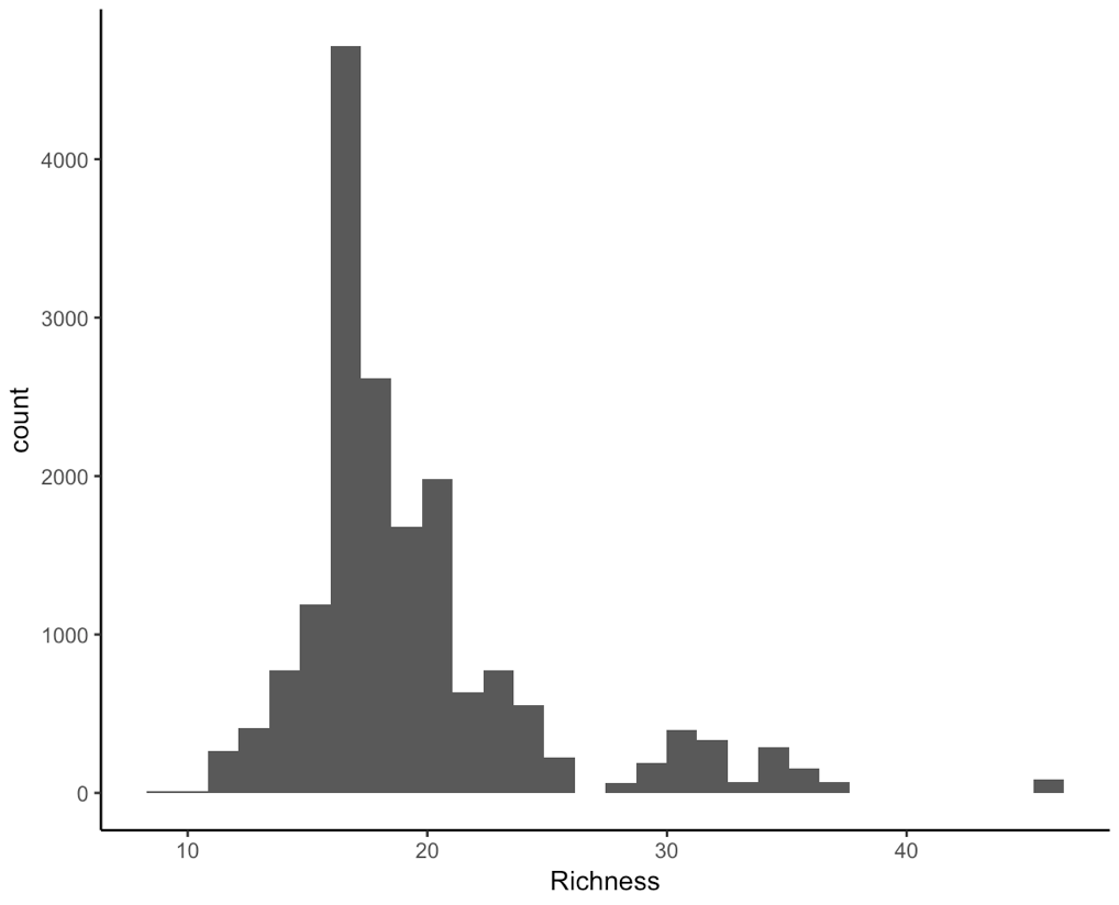
We are working with integers (similar to count data, species only come in whole numbers) and the data are right-skewed, that is because we have a few data points on the extreme right end, they are pulling the mean and median or our data to the right. For ecological data, this is quite common - across all of the sampling plots, we expect that they won’t all have lots of different species within them.

This means that a Poisson distribution might be suitable for our model.

One advantage to fitting models in Stan is that it’s easy to fully take advantage of your computing power. In Stan, we usually run two or more chains - different iterations of our model which we can then compare - if they are massively different, something is not right. If your computer has two or more cores, you can split the chains, i.e., run a chain on each core, saving you some time, as the code will then finish running quicker. This means that you’ll be running the code in parallel.

To enable parallel computing, you can run this line of code and then later on in the model code, you can specify how many cores you want to use.

options(mc.cores = parallel::detectCores())

Now we are all set up for our first model. Remember that the data have a hierarchical structure - species richness is measured in plots, which fall within blocks that are then part of different sites. To derive inferences about changes species richness through time, our models should take this complexity of the data structure into account.

One disadvantage to Stan models is that the code can take a while to finish running, even if we use all of our computer cores, it can still be hours before you can see a summary of your model. Of course, one should use the most suitable type of model for a research question, regardless of how long the model takes to run (within reason…), but in our case, for teaching purposes and so that you can see some model outputs today, we will focus on species richness change within just one of the plots. In that case, the model does not need to include random effects, because on the plot level, there is no replication.

Just so that you know what the syntax looks like and if you have time to wait for this code to finish running, this is how the model for species richness change around Toolik Lake in general would look like:

# Note - this code could take hours to run!
# We are running the model using the default weakly informative priors.
# More about priors coming later in the tutorial!
# stan_lm <- stan_glmer(Richness ~ I(Year-2007) + (1|Site/Block/Plot),
#                     data = toolik_richness, family = poisson,
#                     chains = 4, cores = 4)

# Assess converge by looking at the trace plots
# plot(stan_lm, plotfun = "trace")

# Explore the summary output
# summary(stan_lm)

For teaching purposes only, we will proceed with a model without random effects - that way you can see the outputs of the models as you are going through the tutorial. Note that we do not advise doing this when you are analysing your data for real - of course a model that takes into account the hierarchical structure of the data would be better.

Advantages and disadvantages of using Stan

Stan models can take a long time to compile. One of their key advantage is that you have a lot of freedom to specify the priors (your prior knowledge and expectations of how a given parameter will behave) for your model parameters and you can really account for the complex structure your data might have. There is a time cost to this, as we’ve seen above. One way to approach this is to first make sure your code works on a small chunk of your data, and only afterwards, you can start running the code on the full data (and do other things while you wait for the models to compile).

Now we can run our simplified model. First, let’s check how many years of data we have:

unique(toolik_richness$Year)

There are four years of data from 2008 to 2012. For modelling purposes, it helps to transform the year variable into a continuous variable where the first year is year one, i.e., 2008 is 1, 2009 is 2. That way, the model won’t have to estimate richness in the year 500, the year 501, etc., it will start straight from our first monitoring year.

# Note how now we are using stan_glm because
# there are no random effects
stan_glm1 <- stan_glm(Richness ~ I(Year-2007),
                     data = toolik_richness, family = poisson,
                     chains = 4, cores = 4)

If you find this code still takes a long time, you can change the chains argument to only two chains, but note that it’s better to run models with more than two chains - then you have more room for comparison. If one or more of the four chains is behaving really differently from the rest, then the model might not have converged. What is model convergence? In brief, if a model hasn’t converged, you can’t trust the estimates it gives you. You can find more details in the model design tutorial here.

3. Assessing model convergence

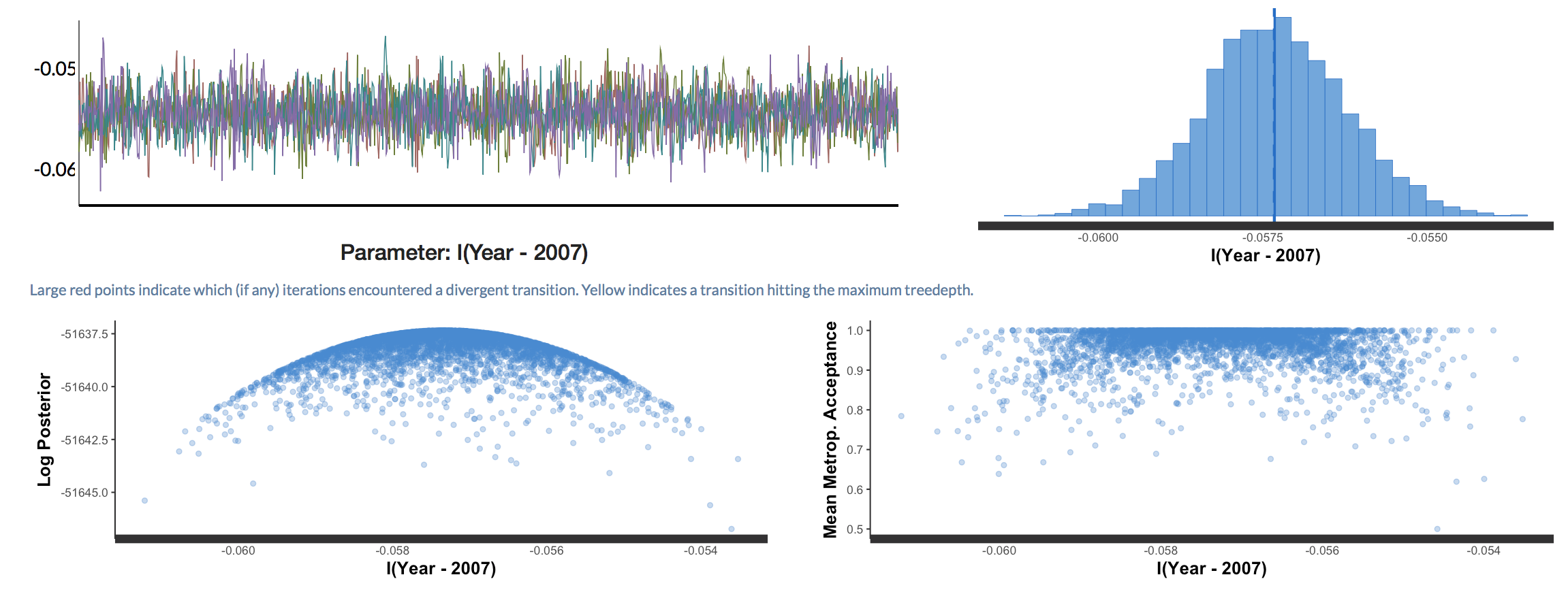
One way to assess model convergence is by visually examining the trace plots. They should be fuzzy with no big gaps, breaks or gigantic spikes.

plot(stan_glm1, plotfun = "trace")

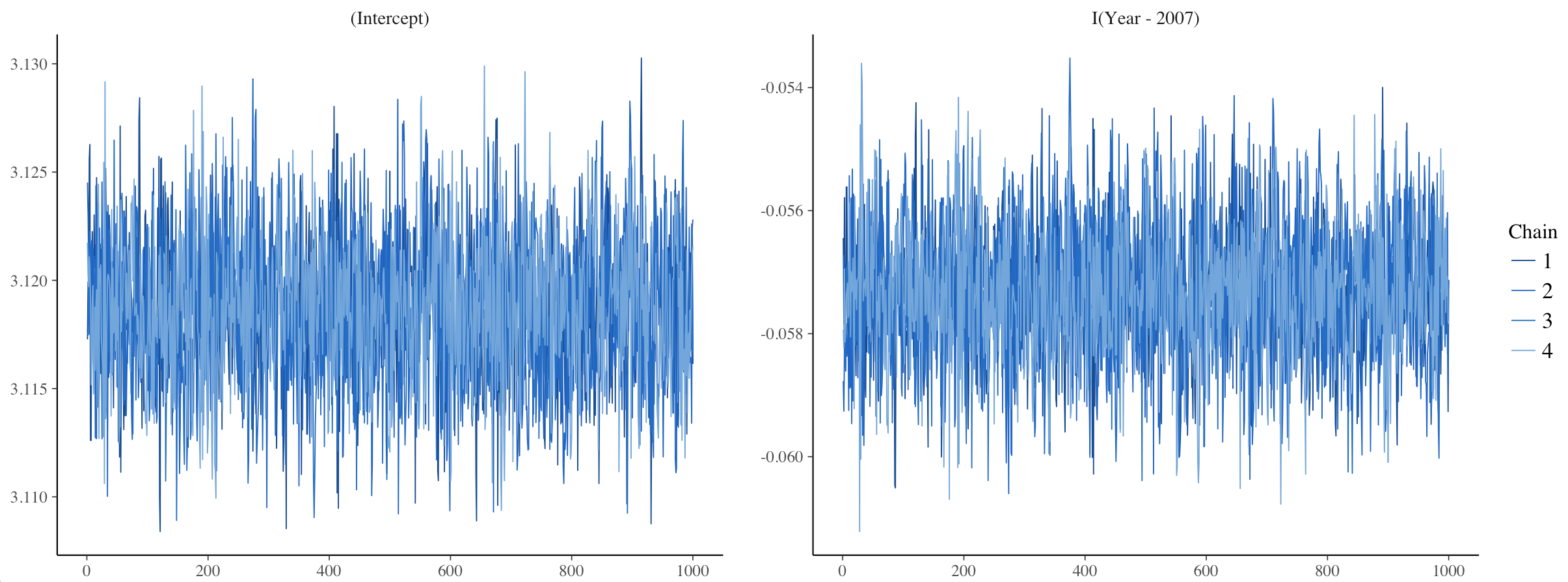
Here, the trace plots look fine.

Next we can look at the summary output.

summary(stan_glm1)

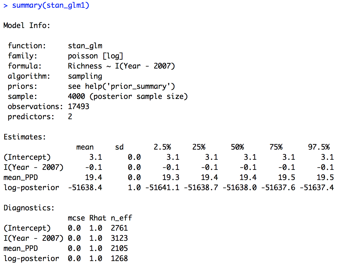
We can see that the effective sample size is alright (there is no hard cut threshold, but more than around 1000 is usually a good sign), another diagnostic metric, the Rhat value is also indicating convergence (an Rhat of 1 is a good sign, more than 1 could indicate trouble).

Posterior predictive checks

The pre-compiled models in rstanarm already include a y_rep variable (our model predictions) in the generated quantities block (your posterior distributions). We can use the pp_check function from the bayesplot package to see how the model predictions compare to the raw data, i.e., is the model behaving as we expect it to be?

pp_check(stan_glm1, plotfun = "stat", stat = "mean")
pp_check(stan_glm1, plotfun = "dens_overlay")

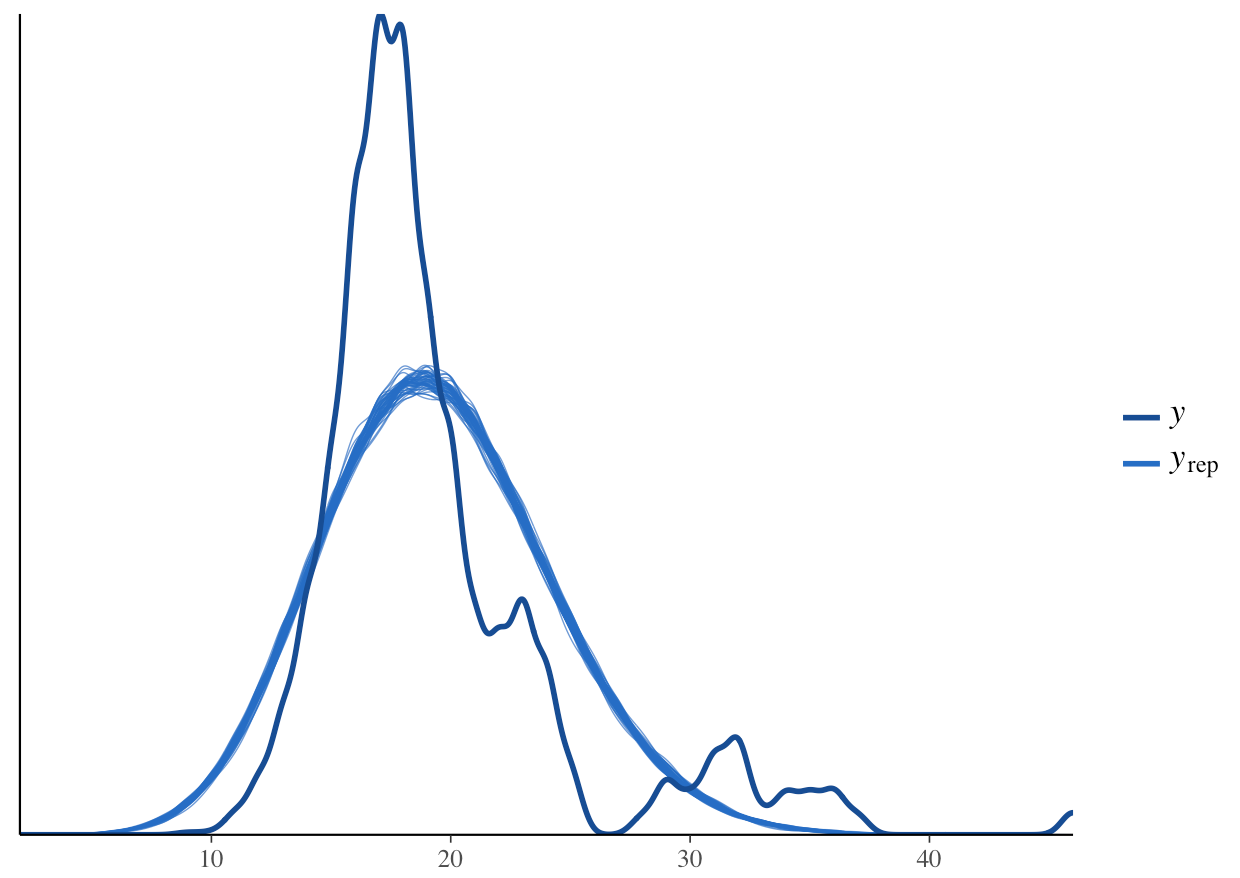
What do you think? How does the density distribution of the model predictions compare with that of the raw data?

From the histogram, we can see that the posterior mean (the dark blue line) aligns well with the raw data. From the density plot, we can see that the model is underpredicting the low species richness value. This is a common problem when working with left-skewed or zero/low number-inflated data. Overall though, the model predictions follow the underlying data, so in summary, we can say that this model fit is acceptable. Note that these decisions can vary based on your question, data and even your statistical philosophy.

Model diagnostics using shinystan

For an interactive exploration of Stan models, you can use the shinystan app. The app is compatible with Stan models generated using the rstan, rstanarm and brms packages, so regardless of how you chooose to run your Stan models, you can still use shinystan to assess whether or not they’ve converged and are behaving properly.

We can launch the app using the code below. That will open a window in our internet browser, where we can further explore our model.

launch_shinystan(stan_glm1)

Have a go at exploring the various options - you’ll probably spot some of the plots we’ve already made in R, but there are many others as well. Here, for example, if there were any divergent chains (i.e. a chain that is behaving in a very weird unexpected way), we would have seen red points. In our case, we don’t have any divergent chains.

Back to our research question:

How has species richness changed over those four years near Toolik lake?

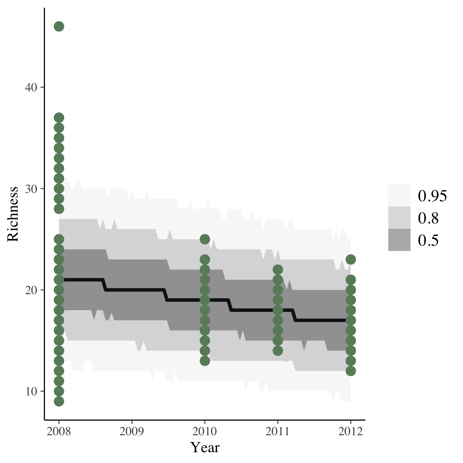
To get the answer, we can plot the model predictions for our model as well as the raw data points.

(model_fit <- toolik_richness %>%
  data_grid(Year = seq_range(Year, n = 101)) %>%
  add_predicted_draws(stan_glm1) %>%
  ggplot(aes(x = Year, y = Richness)) +
  stat_lineribbon(aes(y = .prediction), .width = c(.95, .80, .50),
                  alpha = 1/2, colour = "black") +
  geom_point(data = toolik_richness, colour = "darkseagreen4", size = 3) +
  scale_fill_brewer(palette = "Greys"))

Looks like species richness is decreasing, but also, four years of data is not enough to really test temporal dynamics!

4. Priors

Packages like rstanarm and brms allow us to fit Stan models using simple and quick code syntax. One danger though is that along the way, we might forget to think about our priors! In the code above, we have not specified any priors. In that case, the model uses the default rstanarm priors.

We should check what those are whether they match our expectations of the data.

prior_summary(stan_glm1)

Priors for model 'stan_glm1'
------
Intercept (after predictors centered)
 ~ normal(location = 0, scale = 10)

Coefficients
 ~ normal(location = 0, scale = 2.5)
     **adjusted scale = 1.58

The default priors are normal(0,10) for the intercept and normal(0, 2.5) for the slope. On a first glance, those may seem fairly informative, but it’s important to note that rstanarm automatically centers and scales the data for the model variables (this helps with model convergence), in which case these are weakly informative priors which are suitable for our research question here and the data we have on plant species richness.

If you would like to change the priors, you can add code, for example prior = normal(0, 1), prior_intercept = normal(0, 5) inside the stan_glm() function.

5. Extract Stan code from an rstanarm model

When using packages like rstanarm and brms which you will see in a bit, it’s a good idea to actually look at the Stan code behind the model.

You can extract the code with the following function:

stancode <- rstan::get_stancode(stan_glm1$stanfit)
cat(stancode)

You’ll see a lot of code appear in the console - this is what rstanarm has “written” for you. Amidst the many letters, you can see that the overall structure is like the Stan models we wrote in our intro Stan tutorial - first, we state the parameters for the data, the data gets transformed (scaled and centered), then we define our model and finally, we calculate the predictions in the generated quantities block.

6. Explore a model using a negative binomial distribution

Up until now, we’ve been using a Poisson distribution for our models, which is suitable for when we are working with discrete count data. The Poisson distribution assumes that the mean and variance are the same. In ecology and probably other disciplines too, the data might have variance greater than the mean. In this case, we call the data overdispered. The negative binomial distribution adjusts the variance independently from the mean and as such is more flexible than Poisson. The Poisson distribution is actually a type of a negative binomial distribution.

In rstanarm, it’s easy to update a model using a different data distribution. In our case, we can try a negative binomial distribution.

stan_glm2 <- update(stan_glm1, family = neg_binomial_2)

# Check convergence & priors
plot(stan_glm2, plotfun = "trace")
summary(stan_glm2)
prior_summary(stan_glm2)

# Posterior Predictive Checks
pp_check(stan_glm2, plotfun = "stat", stat = "mean")
pp_check(stan_glm2, plotfun = "dens_overlay")

You can see that the model outputs are very similar - this is to be expected, because the Poisson distribution is actually a type of a negative binomial distribution. Once again, the model is underpredicting the frequency of low species richness values.

7. Run a Stan model using the brms package

brms is another package that serves a similar purpose to rstanarm - it allows you to run Stan models using simple code syntax. brms writes all Stan models from scratch and has to compile them, while rstanarm comes with precompiled code (so when we were running our rstanarm models earlier, you didn’t see any messages about C++ compiling, since that was already done in advance).

The results of the models ran using the different packages should not be different any more than is to be expected by chance (every time you re-run a model using Bayesian inference, the results will be a tiny bit different, because of how the posterior sampling is done, but those differences are of very small magnitudes, like between 0.19887 and 0.19884).

One advantage of brms is that the Stan code you can extract from it is much easier to read than the Stan code coming from rstanarm. We can fit a brms model to check it out.

stan_glm_brms <- brm(bf(Richness ~ I(Year-2007),
                      family = brmsfamily('poisson')), data = toolik_richness,
                   iter = 1000,
                   chains = 4, cores = 4)

summary(stan_glm_brms)
plot(stan_glm_brms)

# Extract Stan code
# The code is nicely annotated, so you can read through
stancode(stan_glm_brms)

Conclusion

In this tutorial we learned to fit Stan models in R using the rstanarm and brms packages which write the Stan code for us, so they can be seen as a gentler introduction to Stan. We looked at two different data distributions that are suitable for left-skewed discrete count data - Poisson and negative binomial. If you are keen to get back into Stan coding, we’ve showed how to extract the Stan code behind the rstanarm and brms models, so you can take that code and develop it further. You can check out our other Stan tutorial. to see how to write and run Stan code using the rstan package.

Further resources

• rstanarm vignette
• brms vignette
• How to Use the rstanarm Package by Jonah Gabry and Ben Goodrich
• Stan website
• Stan manual(v2.14)
• Rstan vignette
• STANCON 2017 Intro Course Materials
• Statistical Rethinking by R. McElreath
• Stan mailing list

Doing this tutorial as part of our Data Science for Ecologists and Environmental Scientists online course?

This tutorial is part of the Stats from Scratch stream from our online course. Go to the stream page to find out about the other tutorials part of this stream!

If you have already signed up for our course and you are ready to take the quiz, go to our quiz centre. Note that you need to sign up first before you can take the quiz. If you haven't heard about the course before and want to learn more about it, check out the course page.

Launch Quiz Centre